Today's class will be held in the BSB Computer Lab (BSB-241). To begin, you will need to read the relevant sections of the instructions "Running Splus at McMaster".
Here is a series of simple exercise to get you started. Try also the examples described in Lecture #03 (trees scatterplot matrices) and Lecture #04 (bivariate frequency polygon). Also, as suggested in Lecture #03, make up a simple data set that will show whether the pairs() function treats missing data pairwise or listwise.Think of some other exercises yourself.
Once you are in the X-win32 window connected to stats, you can launch Splus.
peter@stats[42] # splus
S-PLUS : Copyright (c) 1988, 1998 MathSoft, Inc.
S : Copyright Lucent Technologies, Inc.
Version 5.0 Release 1 for Sun SPARC, SunOS 5.5 : 1998
Working data will be in .
The first time you run Splus, define an object, with a name that is easy to remember, that you will use to specify the size of the graphics window. Note that x11.myterm will still be in your directory the next time you run Splus so you don't have to repeat this step unless you want a different window size. This window will be 500 pixels wide and 375 pixels high.
> x11.myterm <- c("-xrm 'sgraphMotif*canvas.width:500'",
                  "-xrm 'sgraphMotif*canvas.height:375'")
Open a graphics window.
> motif(x11.myterm)
Do a simple calculation.
> (23-4)^2
[1] 361
This time, store the result of the calculation in an object, then display the object.
> result <- (23-4)^2
> result
[1] 361
The object xx will hold a sequence of values running from -3 to +3 in steps of 0.1.
> xx <- seq(-3,3,.1)
> xx
 [1] -3.0 -2.9 -2.8 -2.7 -2.6 -2.5 -2.4 -2.3 -2.2 -2.1 -2.0 -1.9 -1.8 -1.7 -1.6
[16] -1.5 -1.4 -1.3 -1.2 -1.1 -1.0 -0.9 -0.8 -0.7 -0.6 -0.5 -0.4 -0.3 -0.2 -0.1
[31]  0.0  0.1  0.2  0.3  0.4  0.5  0.6  0.7  0.8  0.9  1.0  1.1  1.2  1.3  1.4
[46]  1.5  1.6  1.7  1.8  1.9  2.0  2.1  2.2  2.3  2.4  2.5  2.6  2.7  2.8  2.9
[61]  3.0
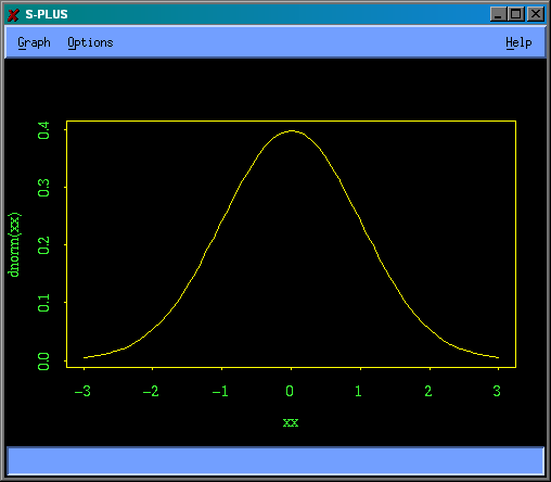
Use the grid of values in xx to plot a graph of the standard normal probability density.
> plot(xx,dnorm(xx), type="l")

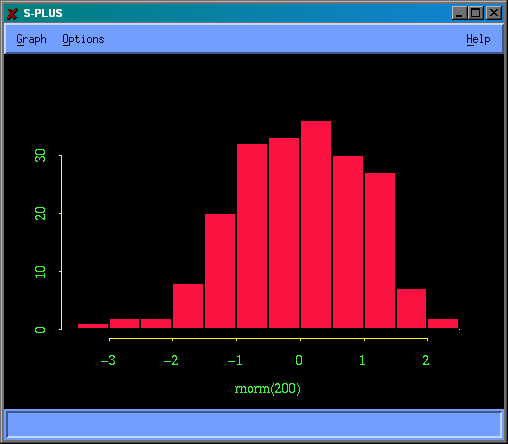
Generate 200 random variates from a standard normal distribution and display them in a histogram.
> hist(rnorm(200))

Display the current directory of Splus objects. Note that x11.myterm is there.
> ls()
 [1] ".Last.value"  ".Random.seed" "a"            "af"           "aff"
 [6] "b"            "f"            "last.dump"    "ma"           "mattt"
[11] "mydata"       "mydatt"       "result"       "state1"       "state2"
[16] "state3"       "state4"       "x11.myterm"   "xx"
Remove two objects you no longer need.
> rm(result, xx)
They are gone.
> ls()
 [1] ".Last.value"  ".Random.seed" "a"            "af"           "aff"
 [6] "b"            "f"            "last.dump"    "ma"           "mattt"
[11] "mydata"       "mydatt"       "state1"       "state2"       "state3"
[16] "state4"       "x11.myterm"
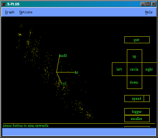
If you created a data frame trees as described in the Lecture #03 notes, you can draw an interactive spinning plot of ht, bnd5, and cci with the spin() function. Because trees is a data frame and spin() only operates on matrices, you need the as.matrix() function to extract the data matrix from trees. Does the spinning plot give you more insight than the scatterplot matrix? What happens if you try to include dbh in a spinning plot, and what can you do about it? Could a spinning plot treat missing data pairwise?
To quit the spin plot, you have to click on the "quit" box with the middle button of a 3-button mouse. To emulate the middle button in X-win32, click on the left and right buttons together.
> spin(as.matrix(trees[ , c(1, 3, 4)]))

> q()