Lab 5: stochastic simulation
Ben Bolker
© 2005 Ben Bolker
1 Static simulation models
1.1 Simple models
1.1.1 Linear model
The code for the static linear model should (I hope)
seem pretty straightforward by now.
I defined an x vector, evenly spaced between
1 and 20; set up parameter values; calculated
a deterministic value; and then added 20
random normally distributed values to the
deterministic values. I then plotted
a scatterplot (plot()) and added
both the theoretical value of the
line (abline in its slope-intercept form)
and the fitted linear regression line
(lm(y~x), as seen in Lab 1).
Pick x values and set parameters:
> x = 1:20
> a = 2
> b = 1
Set random-number seed:
> set.seed(1001)
Calculate the deterministic expectation
(y_det) and then pick 20 normally
distributed values with these means
and s = 2:
> y_det = a + b * x
> y = rnorm(20, mean = y_det, sd = 2)
Plot the simulated values along with
the estimated linear regression line
and the theoretical values:
> plot(x, y)
> abline(lm(y ~ x), lty = 2)
> abline(a, b)
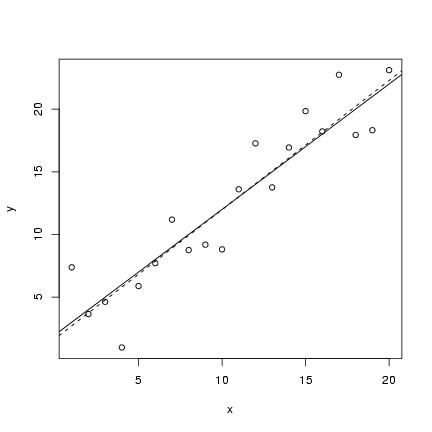 (lines(x,y_det) would have the same
effect as the last statement).
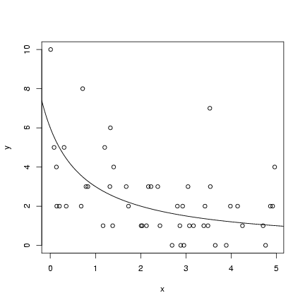
For the hyperbolic simulation:
Pick parameters:
> a = 6
> b = 1
Pick 50 x values uniformly distributed between 0 and 5:
> x = runif(50, min = 0, max = 5)
Calculate the deterministic expectation
(y_det) and then pick 50 Poisson values
with these means:
> y_det = a/(b + x)
> y = rpois(50, y_det)
Plot the simulated values and add the
theoretical curve (we'll wait until Chapter 6
to see how to estimate the curve):
> plot(x, y)
> curve(a/(b + x), add = TRUE)
 Exercise 1:
Simulate a set of 100 values with
- x values uniformly distributed between 0 and 10;
- mean y values following a Ricker model
with a (initial slope) = 1 and b (exponential
decay parameter) = 0.5;
- gamma-distributed heterogeneity with shape parameter 3
and mean as above
Plot the simulated values and superimpose the theoretical
curve.
2 Intermediate simulations
2.1 Pigweed
> set.seed(1001)
> nparents = 50
> noffspr = 10
> L = 30
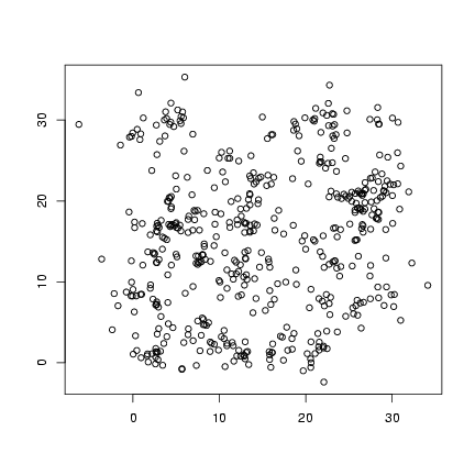
Pick locations of parents:
> parent_x = runif(nparents, min = 0, max = L)
> parent_y = runif(nparents, min = 0, max = L)
Pick angles and distances of offsets of
offspring from parents:
> angle = runif(nparents * noffspr, min = 0, max = 2 * pi)
> dist = rexp(nparents * noffspr, 0.5)
Calculate offspring locations (duplicating each
parent's position noffspr times):
> offspr_x = rep(parent_x, each = noffspr) + cos(angle) * dist
> offspr_y = rep(parent_y, each = noffspr) + sin(angle) * dist
Calculate distances:
> dist = sqrt((outer(offspr_x, offspr_x, "-"))^2 + (outer(offspr_y,
+     offspr_y, "-"))^2)
Calculate neighborhood crowding matrix:
> nbrcrowd = apply(dist < 2, 1, sum) - 1
Plot offspring locations:
> plot(offspr_x, offspr_y, xlab = "", ylab = "")
 Plot distribution of neighborhood crowding:
> b1 = barplot(table(factor(nbrcrowd, levels = 0:max(nbrcrowd)))/length(nbrcrowd),
+     xlab = "Number of neighbors", ylab = "Proportion")
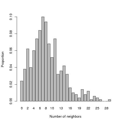 Exercise 2: superimpose a negative binomial
distribution, with the parameters estimated by the method
of moments, on the previous plot.
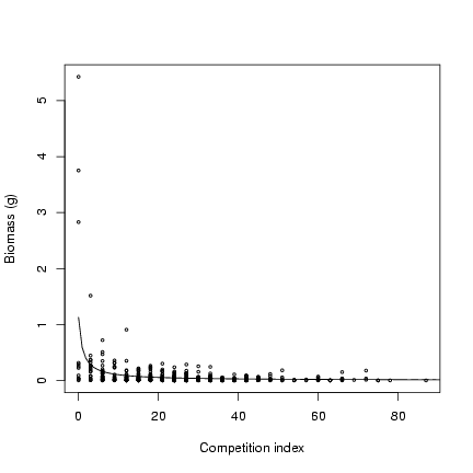
Calculate crowding index as 3 × neighborhood density:
> ci = nbrcrowd * 3
Take parameter of hyperbolic function
and gamma shape parameter from Pacala and Silander:
> M = 2.3
> alpha = 0.49
Expected value of biomass/a (note that
Pacala and Silander estimate the scale parameter
as a function of crowding index, not the mean):
> mass_det = M/(1 + ci)
Pick random deviates:
> mass = rgamma(length(mass_det), scale = mass_det, shape = alpha)
Plot values and theoretical curve:
> plot(ci, mass, cex = 0.5, xlab = "Competition index", ylab = "Biomass (g)")
> curve(M/(1 + x) * alpha, add = TRUE, from = 0)
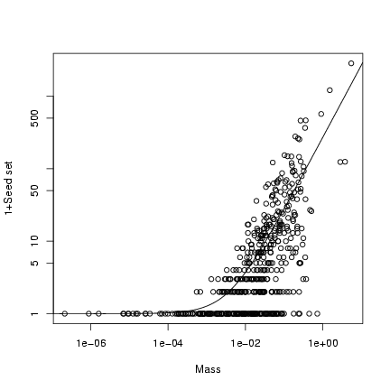
 Parameters for seed set model (slope and overdispersion):
> b = 271.6
> k = 0.569
Deterministic model and random values:
> seed_det = b * mass
> seed = rnbinom(length(seed_det), mu = seed_det, size = k)
Plot (1+seed set) on a double-logarithmic scale:
> plot(mass, 1 + seed, log = "xy", xlab = "Mass", ylab = "1+Seed set")
> curve(b * x + 1, add = TRUE)
 Extra stuff: superimpose the 95% confidence limits on the plot
(use a logarithmically spaced x vector to calculate them):
> logxvec = seq(-7, 0, length = 100)
> xvec = 10^logxvec
> lower = qnbinom(0.025, mu = b * xvec, size = k)
> upper = qnbinom(0.975, mu = b * xvec, size = k)
> lines(xvec, lower + 1, lty = 2)
> lines(xvec, upper + 1, lty = 2)
Exercise 3: superimpose the
median of the distribution on the above graph as well: how
does it differ from the mean?
Exercise 4*: reproduce Figure 3.
or
Exercise 5**: reproduce Figure 3, but with
a beta-binomial error structure instead of a binomial error
structure. Use Morris's parameterization of the beta-binomial,
with p equal to the hyperbolic per capita recruitment
function (R/S=a/(1+(a/b)S) and q = 10.
3 Dynamic models
3.1 Discrete time
3.1.1 Linear growth model
Set up parameters: number of time steps,
starting value, change in N per unit
time (slope), and standard deviations of
process and measurement error:
> nt = 20
> N0 = 2
> dN = 1
> sd_process = sqrt(2)
> sd_obs = sqrt(2)
The first way to do this problem:
marginally less efficient but perhaps
easier to understand, save both
the true and the observed values.
Set aside space:
> Nobs = numeric(nt)
> N = numeric(nt)
Set initial values and pick observation error
for first time step:
> N[1] = N0
> Nobs[1] = N[1] + rnorm(1, sd = sd_obs)
> for (i in 2:nt) {
+     N[i] = N[i - 1] + rnorm(1, mean = dN, sd = sd_process)
+     Nobs[i] = N[i] + rnorm(1, sd = sd_obs)
+ }
An alternative, marginally more efficient way to
run this simulation is keeping only the current value
of N, as follows:
> cur_N = N0
> Nobs[1] = N[1] + rnorm(1, sd = sd_obs)
> for (i in 2:nt) {
+     cur_N = cur_N + rnorm(1, mean = dN, sd = sd_process)
+     Nobs[i] = cur_N + rnorm(1, sd = sd_obs)
+ }
If you plan to experiment a lot with such simulations
with different parameters, it's convenient to define
a function that will do the whole thing in one command
(with default parameters so you can conveniently change
one thing at a time):
> linsim = function(nt = 20, N0 = 2, dN = 1, sd_process = sqrt(2),
+     sd_obs = sqrt(2)) {
+     cur_N = N0
+     Nobs[1] = N[1] + rnorm(1, sd = sd_obs)
+     for (i in 2:nt) {
+         cur_N = cur_N + rnorm(1, mean = dN, sd = sd_process)
+         Nobs[i] = cur_N + rnorm(1, sd = sd_obs)
+     }
+     return(Nobs)
+ }
(make sure that the last statement in your function is
either a variable by itself, or an explicit return() statement)
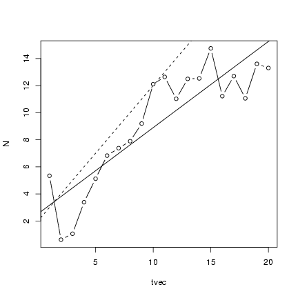
Run one simulation and fit a linear regression:
> N = linsim(sd_proc = 2)
> tvec = 1:20
> lm1 = lm(N ~ tvec)
Plot the points along with the linear regression line
and the theoretical values:
> plot(tvec, N, type = "b")
> abline(lm1)
> abline(a = 2, b = 1, lty = 2)
 Running experiments with many linear simulations:
> nsim = 100
> Nmat = matrix(nrow = 20, ncol = 100)
> for (i in 1:nsim) {
+     Nmat[, i] = linsim()
+ }
Find the 2.5% quantile:
> lower = apply(Nmat, 1, quantile, 0.025)
(You can find both the 2.5% and the 97.5% quantile
at the same time with
t(apply(Nmat,1,quantile,c(0.025,0.975))).)
Exercise 6*:
Using (among other functions) matplot(),
rowMeans(),
quantile() (maybe matlines()):
- run 1000 linear simulations with
sobs=sproc=2.
- Plot all of the individual lines, in gray
- Plot the mean at each time step, in black
- Plot the 95% quantiles at each time step, black, with
dashed lines
Do the results match what you expect from the two extreme
cases (measurement error only/process error only) shown
in the chapter?
3.1.2 Sink population growth model
Here's another example, a model of
a sink population that
is maintained by immigration: the number
of individuals in the population surviving each year is
binomial, with a constant survival probability.
A Poisson-distributed number of immigrants arrives
every year, with a constant rate.
> immigsim = function(nt = 20, N0 = 2, immig, surv) {
+     N = numeric(nt)
+     N[1] = N0
+     for (i in 2:nt) {
+         Nsurv = rbinom(1, size = N[i - 1], prob = surv)
+         N[i] = Nsurv + rpois(1, immig)
+     }
+     return(N)
+ }
Running 1000 simulations:
> nsim = 1000
> nt = 30
> p = 0.95
> N0 = 2
> immig = 10
> Nmat = matrix(ncol = nsim, nrow = nt)
> for (j in 1:nsim) {
+     Nmat[, j] = immigsim(nt = nt, N0 = N0, surv = p, immig = immig)
+ }
> tvec = 1:nt
It turns out that we can also derive the theoretical curve:
E[Nt+1] = p Nt + I,
| |
|
| |
| |
|
|
p(pNt +I) + I = p2 Nt + pI + I |
| |
| |
|
| |
|
So in general, by induction,
|
N(t+n) = pn Nt + |
n-1
�
j=0
|
pj I |
|
or
|
N(t) = pt-1 N1 + |
1-pt-1
1-p
|
I |
|
(accounting for the fact that we start at t=1
and using the formula for the sum of a geometric series,
�j=0n-1 pj = (1-pt-1)/(1-p)).
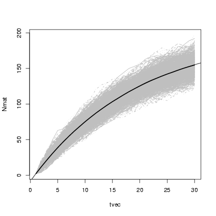
Plotting x
and superimposing
lines showing the mean value of the simulations:
> matplot(tvec, Nmat, type = "l", col = "gray")
> lines(tvec, rowMeans(Nmat), lwd = 2)
> curve(p^(x - 1) * N0 + (1 - p^(x - 1))/(1 - p) * immig, add = TRUE)
3.2 Continuous time
Solving the theta-logistic model,
|
|
dN
dt
|
= rN |
�
�
|
1- |
N
K
|
�
�
|
q
|
|
|
numerically:
Attach odesolve package:
> library(odesolve)
Define a function for the derivative. It must
have arguments (time, state vector, parameters), although
they need not be called t, y, params.
The only other peculiarity is that instead of returning
the derivative (dNdt in this case)
by itself you actually have to return a list
containing the derivative as its first element and
"a vector of global values that are required at each point"
(which can usually be NULL).
> derivfun = function(t, y, parms) {
+     r = parms[1]
+     K = parms[2]
+     theta = parms[3]
+     N = y[1]
+     dNdt = r * N * sign(1 - N/K) * abs((1 - N/K))^theta
+     list(dNdt, NULL)
+ }
Once you've defined the derivative function, you can
use the lsoda function to solve
that differential equation for any set of
starting values (y),
times (times), and parameters (parms)
you like.
> tvec = seq(0, 50, by = 0.2)
> x1 = lsoda(y = c(N = 1), times = tvec, func = derivfun, parms = c(r = 0.2,
+     K = 10, theta = 1))
You get back a numeric matrix with a column for
the times and columns for all of the state variables
(only one in this case):
> head(x1)
     time        N
[1,]  0.0 1.000000
[2,]  0.2 1.036581
[3,]  0.4 1.074341
[4,]  0.6 1.113303
[5,]  0.8 1.153495
[6,]  1.0 1.194945
Re-running the solution for different values of q:
> x2 = lsoda(y = c(N = 1), times = tvec, func = derivfun, parms = c(r = 0.2,
+     K = 10, theta = 2))
> x3 = lsoda(y = c(N = 1), times = tvec, func = derivfun, parms = c(r = 0.2,
+     K = 10, theta = 0.5))
Putting the results together into a single matrix
(both columns of the first matrix and only the
second column of the other two):
> X = cbind(x1, x2[, "N"], x3[, "N"])
Plotting with matplot(),
and using curve and the known
solution for the plain old logistic
to check the solution when q = 1:
> matplot(X[, "time"], X[, 2:4], type = "l", col = 1, xlab = "time",
+     ylab = "N")
> r = 0.2
> K = 10
> N0 = 1
> curve(K/((1 + (K/N0 - 1) * exp(-r * x))), type = "p", add = TRUE)
> legend(30, 4, c(expression(theta == 1), expression(theta == 2),
+     expression(theta == 0.5)), lty = 1:3)
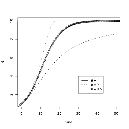 (remember you have to use == to
get an equals sign in a
math expression).
4 Power etc. calculations
This section will first go through a relatively
simple example (the source-sink population model
presented above), showing the basic steps of a
power calculation. I'll then give a briefer sketch
of some of the gory details of doing the Shepherd model
power analysis discussed in the chapter.
4.1 Sink population dynamics
The sink population presented above was a recovering
sink population: the biological question I will
try to answer is: how long do I have to sample the
population for to test that it is really recovering?
How does this depend on the survival and immigration
rates?
First, simulate one set of values and a time vector:
> nt = 20
> sim0 = immigsim(nt = nt, N0 = 2, surv = 0.9, immig = 10)
> tvec = 1:nt
Run a linear regression and extract the
point estimate
and confidence limits
for the slope:
> lm1 = lm(sim0 ~ tvec)
> slope = coef(lm1)["tvec"]
> ci.slope = confint(lm1)["tvec", ]
(look at the output of confint(lm1) to see how it's structured).
Now run the model for a series of lengths of observation time
and record the values for each length:
> nvec = c(3, 5, 7, 10, 15, 20)
> nsim = 500
> powsimresults = matrix(nrow = length(nvec) * nsim, ncol = 5)
> colnames(powsimresults) = c("n", "sim", "slope", "slope.lo",
+     "slope.hi")
> ctr = 1
> for (i in 1:length(nvec)) {
+     nt = nvec[i]
+     tvec = 1:nt
+     cat(nt, "\n")
+     for (sim in 1:nsim) {
+         current.sim = immigsim(nt = nt, N0 = N0, surv = p, immig = immig)
+         lm1 = lm(current.sim ~ tvec)
+         slope = coef(lm1)["tvec"]
+         ci.slope = confint(lm1)["tvec", ]
+         powsimresults[ctr, ] = c(nt, sim, slope, ci.slope)
+         ctr = ctr + 1
+     }
+ }
3
5
7
10
15
20
A couple of R tricks in this code:
- I'm going to keep the output in long format, with
each row containing the sample size and simulation number
along with the estimate and confidence intervals:
this will make it easy to cross-tabulate the results
(see below)
- I keep a counter variable ctr to track
which row of the matrix I'm filling in, and add
one to it each time through the loop. (Alternately
I could calculate that at the ith sample size
and sth simulation I should be filling in
row (i-1)*nsim+i.)
Make sure to reset ctr if you re-run the
for loops.
- the cat() command is just printing results
as I go along: on Windows you may have to go to a menu
and unselect the "buffered output" option. The
"\n" at the end specifies a new line.
- I keep track of simulation number in the loop
but the index of the sample size:
i is (1, 2, 3, ...) rather
than i (3, 5, 7, ...). This isn't
totally necessary in this case since we're using
ctr to index the rows of the matrix, but it's
generally safer.
Now summarize the results, cross-tabulating
by the number of samples.
> nfac = factor(powsimresults[, "n"])
Select the point estimate and calculate its mean
(E[[^s]])
for each observation length:
> slope.mean = tapply(powsimresults[, "slope"], nfac, mean)
Calculate the standard deviation:
> slope.sd = tapply(powsimresults[, "slope"], nfac, sd)
to calculate the variance of the estimate.
Calculating whether the true value fell within
the confidence limits in a particular simulation.
(The theoretical value of the slope is a little
hard here since the expected value of the population
is actually to grow to an asymptote. Near the
beginning the slope is close to the immigration
rate:
> ci.good = (powsimresults[, "slope.hi"] > immig) & (powsimresults[,
+     "slope.lo"] < immig)
Calculating the coverage by cross-tabulating the number of "good" confidence
intervals and dividing by the number of simulations per d/sample size combination:
> nsim = 500
> slope.cov = tapply(ci.good, nfac, sum)/nsim
(so the "coverage" actually decreases in this case,
but this is a bad example - sorry!)
Calculating whether the null value (zero) did not
fall within the confidence limits:
> null.value = 0
> reject.null = (powsimresults[, "slope.hi"] < null.value) | (powsimresults[,
+     "slope.lo"] > null.value)
Calculating the power by cross-tabulating the number of rejections
of the null hypothesis and dividing by the number of simulations per d/sample size combination:
> slope.pow = tapply(reject.null, nfac, sum)/nsim
In this case it's very easy to see, very quickly, that
the population is recovering ...
Exercise 7*: redo this example, but with negative
binomial growth (with k=5, k=1, and k=0.5). If you want
to be fancy, try to nest an additional for loop and
cross-tabulate your answers with a single command (see code
below under reef fish example): otherwise simply change
the variable and re-run the code three times.
or
Exercise 8**: in R, you
can fit a quadratic function with
> lm.q = lm(sim0 ~ tvec + I(tvec^2))
Extract the point estimate
for the quadratic term
with coef(lm.q)[3] and
the confidence intervals with
confint(lm.q)[3,].
For the original model (with Poisson variability),
do a power analysis of your ability to
detect the leveling-off of the
curve (as a negative
quadratic term in the regression fit)
as a function of number of observation
periods. (If you're really ambitious,
combine the two problems and
try this with negative binomial variation.)
4.2 Reef fish dynamics
Regenerating a simulated version of Schmitt et al. data.
(Re)define zero-inflated negative binomial and Shepherd functions:
> rzinbinom = function(n, mu, size, zprob) {
+     ifelse(runif(n) < zprob, 0, rnbinom(n, mu = mu, size = size))
+ }
> shep = function(x, a = 0.696, b = 9.79, d = 1) {
+     a/(1 + (a/b) * x^d)
+ }
Parameters for distribution of settlers
(m, k, pz) and
Shepherd function (a, b, d):
> mu = 25.32
> k = 0.932
> zprob = 0.123
> a = 0.696
> b = 9.79
> d = 1.1
> n = 603
Simulate one set of values:
> set.seed(1002)
> settlers = rzinbinom(n, mu = mu, size = k, zprob = zprob)
> recr = rbinom(n, prob = shep(settlers, a, b, d), size = settlers)
The nonlinear least-squares function nls() takes
a formula and a named set of starting values.
Start by fitting the Beverton-Holt, which is easier
to fit than the Shepherd.
(This is a typical way to fit a complex model: start with
a simpler, easier-to-fit model that is a special case of the complex model,
then use those fitted parameters as a starting point
for the harder estimation problem.)
Use the theoretical
values of a and b as starting parameters
for the Beverton-Holt fit:
> bh.fit = nls(recr ~ a * settlers/(1 + (a/b) * settlers), start = c(a = 0.696,
+     b = 9.79))
> bh.fit
Nonlinear regression model
  model:  recr ~ a * settlers/(1 + (a/b) * settlers)
   data:  parent.frame()
        a         b
0.7775758 6.6934193
 residual sum-of-squares:  1639.527
The function coef(bh) gives the fitted parameters
(coefficients). Use these, plus a starting value of d=1,
to fit the Shepherd function.
> shep.fit = nls(recr ~ a * settlers/(1 + (a/b) * settlers^d),
+     start = c(coef(bh.fit), d = 1))
> shep.fit
Nonlinear regression model
  model:  recr ~ a * settlers/(1 + (a/b) * settlers^d)
   data:  parent.frame()
         a          b          d
 0.5998674 12.0196853  1.1362227
 residual sum-of-squares:  1631.212
Calculate confidence intervals:
> ci = confint(shep.fit)
Waiting for profiling to be done...
> ci
       2.5%      97.5%
a 0.4630841  0.8419771
b 6.2920786 26.0900580
d 0.9846074  1.3152524
Extract the estimates for d:
> ci["d", ]
     2.5%     97.5%
0.9846074 1.3152524
Sometimes the confidence interval fitting runs into trouble
and stops with an error like
Error in prof$getProfile() : step factor 0.000488281 reduced
    below 'minFactor' of 0.000976562
This kind of glitch is fairly rare when doing analyses one at a time,
but very common when doing power analyses, which require thousands
or tens of thousands of fits. A few R tricks for dealing with this:
- x = try(command) "tries" a command to see if it works or not;
it it doesn't work, Rdoesn't stop but sets x equal to the
error message. To test whether the command stopped or not, see if
class(x)=="try-error"
- while and if are commands for flow control
(like the for() command introduced earlier in this lab):
if executes a set of commands (once) if some condition
is true, and
while loops and executes a set of commands as long as some condition
is true
The code below is a slightly simplified version of what I did
to generate the values
> getvals = function(n = 100, d = 1) {
+     OK = FALSE
+     while (!OK) {
+         z = simdata(n, d)
+         bh.fit = try(nls(recr ~ a * settlers/(1 + (a/b) * settlers),
+             start = c(a = 0.696, b = 9.79), data = z))
+         shep.fit = try(nls(recr ~ a * settlers/(1 + (a/b) * settlers^d),
+             start = c(coef(bh.fit), d = 1), data = z))
+         OK = (class(shep.fit) != "try-error" && class(bh.fit) !=
+             "try-error")
+         if (OK) {
+             bh.ci = try(confint(bh.fit))
+             shep.ci = try(confint(shep.ti))
+             OK = (class(shep.ci) != "try-error" && class(bh.ci) !=
+                 "try-error")
+         }
+     }
+     res = c(coef(bh.fit), bh.ci, coef(shep.fit), shep.ci)
+     names(res) = c("a.bh", "b.bh", "a.bh.lo", "b.bh.lo", "a.bh.hi",
+         "b.bh.hi", "a.shep", "b.shep", "d.shep", "a.shep.lo",
+         "b.shep.lo", "d.shep.lo", "a.shep.hi", "b.shep.hi", "d.shep.hi")
+     res
+ }
Here I loaded the results of a big set of simulations I had run:
download it from the web page if you want to actually run these commands.
> load("chap5-batch2.RData")
I then used
> faclist = list(factor(resmat[, "d"]), factor(resmat[, "n"]))
To define a set of factors to break up the data (i.e., I will want
to cross-tabulate by both true parameter value d and sample size)
and then ran
> d.shep.mean = tapply(resmat[, "d.shep"], faclist, mean)
to calculate the mean value E[[^d]] and
> d.shep.sd = tapply(resmat[, "d.shep"], faclist, sd)
to calculate the variance of the estimate.
Calculating whether the true value fell within
the confidence limits in a particular simulation:
> ci.good = (resmat[, "d.shep.hi"] > resmat[, "d"]) & (resmat[,
+     "d.shep.lo"] < resmat[, "d"])
Calculating the coverage by cross-tabulating the number of "good" confidence
intervals and dividing by the number of simulations per d/sample size combination:
> nsim = 400
> d.shep.cov = tapply(ci.good, faclist, sum)/nsim
Calculating whether the null value did not
fall within the confidence limits:
> null.value = 1
> reject.null = (resmat[, "d.shep.hi"] < null.value) | (resmat[,
+     "d.shep.lo"] > null.value)
Calculating the power by cross-tabulating the number of null-hypothesis
rejections and dividing by the number of simulations per d/sample size combination:
> nsim = 400
> d.shep.pow = tapply(reject.null, faclist, sum)/nsim
Randomization tests (to come)
File translated from
TEX
by
TTH,
version 3.67.
On 6 Oct 2005, 16:11.
 (lines(x,y_det) would have the same
effect as the last statement).
For the hyperbolic simulation:
Pick parameters:
 Exercise 1:
Simulate a set of 100 values with
 Plot distribution of neighborhood crowding:
 Exercise 2: superimpose a negative binomial
distribution, with the parameters estimated by the method
of moments, on the previous plot.
Calculate crowding index as 3 × neighborhood density:
 Parameters for seed set model (slope and overdispersion):
 Extra stuff: superimpose the 95% confidence limits on the plot
(use a logarithmically spaced x vector to calculate them):
 Running experiments with many linear simulations:

 (remember you have to use == to
get an equals sign in a
math expression).