Lab 3: solutions
© 2005 Ben Bolker
Exercise 1*:
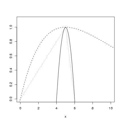
- Quadratic: easiest to construct in the
form (y=-(x-a)2+b), where a is the location
of the maximum and b is the height.
(Negative sign in front of the quadratic term
to make it curve downward.)
Thus a=5, b=1.
- Ricker: if y=axe-bx, then
(as discussed in the chapter) the location
of the maximum is at x=1/b and the height
is at a/(be). Thus b=0.2, a=0.2*e.
- Triangle: let's say for example
that the first segment is a line with
intercept zero and slope 1/5, and the second
segment has equation -1*(x-5)+1.
> curve(-(x - 5)^2 + 1, from = 0, to = 10, ylim = c(0, 1.1), ylab = "")
> curve(0.2 * exp(1) * x * exp(-0.2 * x), add = TRUE, lty = 2)
> curve(ifelse(x < 5, x/5, -(x - 5) + 1), add = TRUE, lty = 3)
 What else did you try? (Sinusoid, Gaussian
(exp(-x2)), ?)
Exercise 2*:
What else did you try? (Sinusoid, Gaussian
(exp(-x2)), ?)
Exercise 2*:
|
n(t) = |
K
|
1+ |
ć
č
|
K
n(0)
|
-1 |
ö
ř
|
exp(-r t) |
|
|
|
Since n(0) << 1 (close to zero, or much less than 1),
K/n(0)-1 » K/n(0). So:
Provided t isn't too big,
K/n(0) exp(-rt) is also a lot larger than 1,
so
Now multiply top and bottom by n(0)/K exp(rt)
to get the answer.
Exercise 3*:
When b=1, the Shepherd function
reduces to RN/(1+aN), which is a form
of the M-M.
You should try not to be confused by the fact
that earlier in class we used the form
ax/(b+x) (asymptote=a, half-maximum=b);
this is just a different parameterization
of the function. To be formal about it, we could
multiply the numerator and denominator of
RN/(1+aN) by 1/a to get our
equation in the form (R/a) N / ((1/a) + N),
which matches what we had before with a=R/a,
b=1/a.
Near 0:
we can do this either by evaluating the derivative
S˘(N) at N=0 (which gives R - see below) or by taking the limit
of the whole function S(N) as N ® 0, which gives
RN (because the aN
term in the denominator becomes small relative to 1),
which is a line through the origin with slope R.
For large N:
if b=1, we know already that this is Michaelis-Menten,
and in this parameterization the asymptote is R/a (in the limit,
the 1 in the denominator becomes irrelevant and the function becomes
approximately [RN/aN]=[R/a]). If b is not 1 (we'll
assume it's greater than 0) we can
start the same way (1+aN » aN), but now we have RN/(aN)b.
Write this as [R/(ab)] N(1-b). If b > 1,
N is raised to a negative
power and the function goes to zero as N ® Ą. If b < 1,
N is raised to a positive power and R(N) approaches infinity
as N ® Ą
(it never levels off).
If b=0 then the function is just a straight line (no asymptote),
with slope R/2.
We don't really need to calculate the slope (we can figure out
logically that it must be negative but decreasing in magnitude for
large N and b > 1; positive and decreasing to 0 when b=1; and
positive and decreasing, but never reaching 0, when b > 1. Nevertheless,
for thoroughness (writing this as a product and using the
product, power, and chain rules):
| |
|
|
R (1+aN)-b + RN ·-b (1+aN)(-b-1) a |
| | (1) |
| |
|
|
R (1+aN)-b -abRN (1+aN)(-b-1) |
| | (2) |
| |
|
|
R (1+aN)-b-1 ( (1+aN) -abN ) |
| | (3) |
| |
|
| R (1+aN)-b-1 (1+aN (1-b)) |
| | (4) |
|
You could also do this by the quotient rule.
The derivative of the numerator is R (easy); the
derivative of the denominator is b ·(1+aN)b-1 ·a = ab (1+aN)b-1 (power rule/chain rule).
| |
|
|
|
g(N) f˘(N) - f(N) g˘(N)
( g(N) )2
|
|
| | (5) |
| |
|
|
|
R (1+aN)b - RN (ab (1+aN)b-1 )
( 1+ aN )2b
|
|
| | (6) |
| |
|
|
R (1+aN)b-1 ( 1+aN - abN )
( 1+ aN )2b
|
|
| | (7) |
|
You can also do this with R (using D()),
but it won't simplify the expression for you:
> dS = D(expression(R * N/(1 + a * N)^b), "N")
> dS
R/(1 + a * N)^b - R * N * ((1 + a * N)^(b - 1) * (b * a))/((1 +
    a * N)^b)^2
If you want to know the value for a particular N,
and parameter values,
use eval() to evaluate the expression:
> eval(dS, list(a = 1, b = 2, R = 2, N = 2.5))
[1] -0.06997085
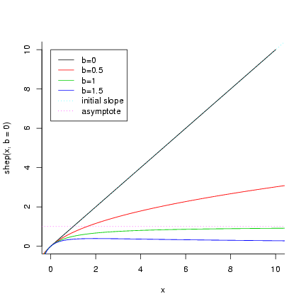
A function to evaluate the Shepherd (with
default values R=1, a=1, b=1):
> shep = function(x, R = 1, a = 1, b = 1) {
+     R * x/(1 + a * x)^b
+ }
Plotting:
> curve(shep(x, b = 0), xlim = c(0, 10), bty = "l")
> curve(shep(x, b = 0.5), add = TRUE, col = 2)
> curve(shep(x, b = 1), add = TRUE, col = 3)
> curve(shep(x, b = 1.5), add = TRUE, col = 4)
> abline(a = 0, b = 1, lty = 3, col = 5)
> abline(h = 1, col = 6, lty = 3)
> legend(0, 10, c("b=0", "b=0.5", "b=1", "b=1.5", "initial slope",
+     "asymptote"), lty = rep(c(1, 3), c(4, 2)), col = 1:6)
 extra credit: use the expression above for
the derivative, and look just at the numerator.
When does (1+aN-abN)=(1+a (1-b)N) = 0? If b Ł 1
the whole expression must always be positive (a ł 0, N ł 0).
If b > 1 then we can solve for N:
extra credit: use the expression above for
the derivative, and look just at the numerator.
When does (1+aN-abN)=(1+a (1-b)N) = 0? If b Ł 1
the whole expression must always be positive (a ł 0, N ł 0).
If b > 1 then we can solve for N:
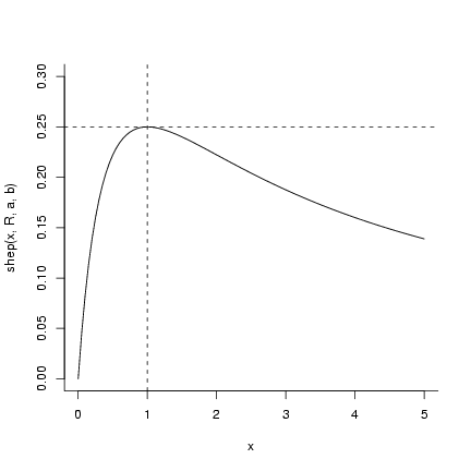
When N=1/(a(b-1)), the value of the function is
R/(a ·(b-1) ·(1+1/(b-1))b) (for b=2
this simplifies to R/(4a)).
> a = 1
> b = 2
> R = 1
> curve(shep(x, R, a, b), bty = "l", ylim = c(0, 0.3), from = 0,
+     to = 5)
> abline(v = 1/(a * (b - 1)), lty = 2)
> abline(h = R/(a * (b - 1) * (1 + 1/(b - 1))^b), lty = 2)
 There's actually another answer that we've missed by
focusing on the numerator.
As N ® Ą, the
limit of the derivative is
There's actually another answer that we've missed by
focusing on the numerator.
As N ® Ą, the
limit of the derivative is
|
|
R (aN)b-1 (a(1-b) N)
(aN)2b
|
= |
R (1-b)
(aN)b
|
; |
|
R > 0, (1-b) < 0 for b > 1, aN > 0, so the
whole thing is negative and decreasing in magnitude
toward zero.
Exercise 4*:
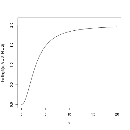
Holling type III functional response, standard parameterization:
f(x)=ax2/(1+bx2).
Asymptote: as x®Ą, bx2+1 » bx2 and
the function approaches a/b.
Half-maximum:
So, if we have asymptote A=a/b
and half-max H=Ö{1/b},
then b=1/H2 and a=Ab=A/H2.
So
which might be more simply written as
A(x/H)2/(1+(x/H)2).
Check with a plot:
> holling3 = function(x, A = 1, H = 1) {
+     A * (x/H)^2/(1 + (x/H)^2)
+ }
> curve(holling3(x, A = 2, H = 3), from = 0, to = 20, ylim = c(0,
+     2.1))
> abline(h = c(1, 2), lty = 2)
> abline(v = 3, lty = 2)
 Exercise 5*:
Population-dynamic:
Exercise 5*:
Population-dynamic:
|
n(t) = |
K
|
1+ |
ć
č
|
K
n(0)
|
-1 |
ö
ř
|
exp(-r t) |
|
|
|
Asymptote K, initial exponential slope r,
value at t=0 n(0),
derivative at t=0 r n(0) (1-n(0)/K).
Statistical:
Asymptote 1, value at x=0 exp(a)/(1+exp(a)).
The easiest way to figure this out is first to set
K=1 and multiply the population-dynamic version by
exp(rt)/exp(rt):
|
n(t) = |
exp(rt)
|
exp(rt) + |
ć
č
|
1
n(0)
|
-1 |
ö
ř
|
|
|
|
and multiply the statistical version by
exp(-a)/exp(-a):
|
f(x) = |
exp(bx)
exp(-a) + exp(bx)
|
|
|
This manipulation makes it clear (I hope) that
b=r, x=t, and (1/n(0)-1)=exp(-a), or
a=-log(1/n(0)-1), or n(0)=1/(1+exp(-a)).
Set up parameters and equivalents:
> a = -5
> b = 2
> n0 = 1/(1 + exp(-a))
> n0
[1] 0.006692851
> K = 1
> r = b
Draw the curves:
> curve(exp(a + b * x)/(1 + exp(a + b * x)), from = 0, to = 5,
+     ylab = "")
> curve(K/(1 + (K/n0 - 1) * exp(-r * x)), add = TRUE, type = "p")
> legend(0, 1, c("statistical", "pop-dyn"), pch = c(NA, 1), lty = c(1,
+     NA), merge = TRUE)
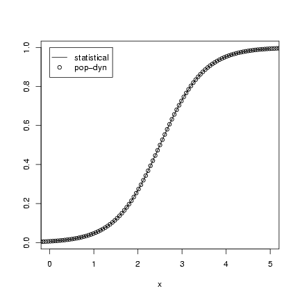 The merge=TRUE statement in the
legend() command makes R plot the
point and line types in a single column.
The merge=TRUE statement in the
legend() command makes R plot the
point and line types in a single column.
File translated from
TEX
by
TTH,
version 3.67.
On 14 Sep 2005, 16:37.