EDA means "Exploratory Data Analysis."
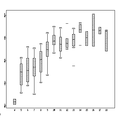
The age-length relationship defines the growth curve. What does it look like? How many ages are present in the data? How variable is length at each age? To begin with, I used the data with all sites and all year classes combined. I could have used plot(fage, flen); what were the advantages of using boxplots here?
> boxplot(split(flen, fage))

How does the growth increment vary with age? For now, I am ignoring differences between year classes and sites. Later, of course, we will want to look for differences between sites, to measure the effect of the effluent, and we may want to allow for differences between year classes, since fish spawned in different years will pass through a given age in different years and hence under possibly different growing conditions.
> boxplot(split(ingrow, inage))
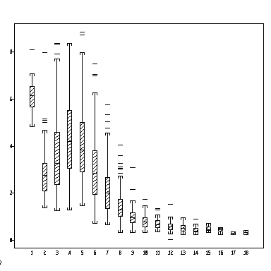
Note how the increment becomes smaller and less variable as the fish get older. This suggests that we should be working with log-transformed growth increments. Why? Try taking logs and see how the graph changes.
> boxplot(split(log(ingrow), inage))
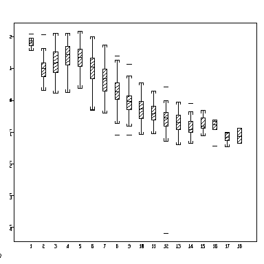
Do you notice an outlier? Find out which fish it came from and investigate it. Was it an outlier before I transformed the data? Does it matter? I suppose I should have continued working with log(ingrow) instead of ingrow, but I will try that in another session.
How does the growth increment in age 4 vary from year to year?
> boxplot(split(ingrow[inage==4],ygrow[inage==4]))
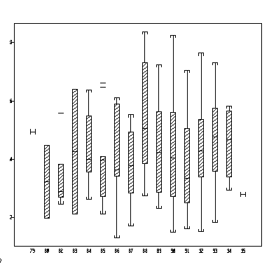
What if we only consider fish upstream from the pollution source?
> boxplot(split(ingrow[inage==4 & site=="up2"],ygrow[inage==4 & site=="up2"]))
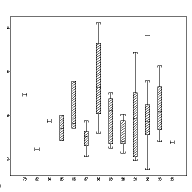
Make a new data frame to focus on year-4 growth of fish sampled at age 7. Why do I need the last comma? What was the advantage in making a new data frame?
> operctmp <- operc[fage==7 & inage==4,]
Since I didn't attach the new data frame, I have to prefix its variable names with operctmp$, otherwise S will take the variable names from the attached data frame. What happens if I attach more than one data frame? Would this have been OK to do?
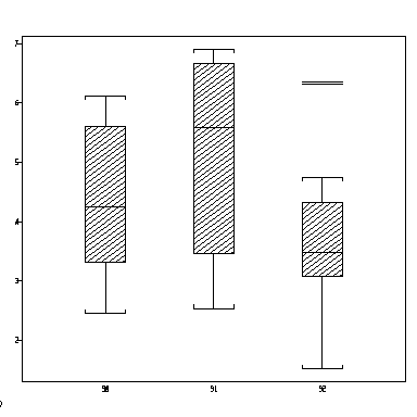
> boxplot(split(operctmp$ingrow[site=="downff"],operctmp$ygrow[site=="downff"]))
We are now getting very specific: this plot shows how the age-4 growth increment varies between fish and between years, for fish sampled 15 km below the pulp mill at age 7. Looking at this chart reminds me that the summer of 1992 was very cold and wet in Northern Ontario! It looks as though we will have to adjust for year in all the analyses.
How does the age distribution vary between sites?
> table(fage,site)
   downff downtb up2
 4      4      0   4
 5     30     35  30
 6     48     90  72
 7     56     84 126
 8     40    104  80
 9    108     54  90
10    110     60  60
11     44    121  66
12     12     48  24
13     26     52  26
14     56     28   0
15      0     30  15
16     16     16   0
17      0     34   0
18      0     36  18
These examples should get you started. Be creative... ask interesting questions and see how you can use S to answer them.