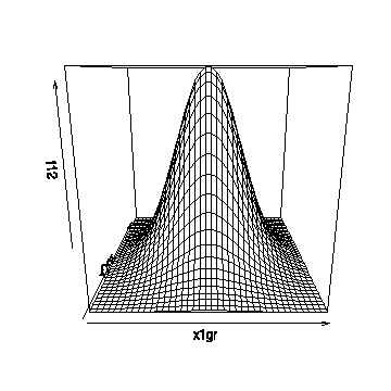
Here are three different ways to compute the bivariate standard normal density function over a regular two-dimensional grid defined by x1gr in the x1 direction and x2gr in the x2 direction. The persp() function is then called to draw a perspective plot.
The first way initializes a matrix to hold the result, then uses nested for loops to compute the density at each grid point (x1, x2).
> bivnormplot
function (x1gr, x2gr)
{
    f12 <- matrix(0, nrow = length(x1gr), ncol = length(x2gr))
    i1 <- 0
    for (x1 in x1gr) {
        i1 <- i1 + 1
        i2 <- 0
        for (x2 in x2gr) {
            i2 <- i2 + 1
            f12[i1, i2] <- (1/(2*pi))*exp(-0.5*(x1^2 + x2^2))
        }
    }
    persp(x1gr, x2gr, f12)
    invisible()
}
Here is how bivnormplot() is used. In this example the grid goes from -3 to 3 in 40 steps in each direction. The graph shown here was drawn in R; it will look a bit different in Splus. You could add other parameters to the call to persp() if you wanted to change the viewing angle, add shading, etc.
> bivnormplot(seq(-3,3,len=40),seq(-3,3,len=40))
The second way uses expand.grid() to create a matrix with two columns holding all the (x1, x2) pairs from the grid, then computes the matrix of density values without having to use a for() loop.
> bivnormplota
function (x1gr, x2gr)
{
    x12gr <- expand.grid(list(x1gr, x2gr))
    f12 <- matrix((1/(2 * pi)) * exp(-0.5 * (x12gr[, 1]^2 + x12gr[,
        2]^2)), nrow = length(x1gr))
    persp(x1gr, x2gr, f12)
    invisible()
}

> bivnormplota(seq(-3,3,len=40),seq(-3,3,len=40))
The result is not shown here as it is exactly the same as given by bivnormplot(). If you want to understand this code better, you should explore expand.grid() to see exactly what it does.
The third way uses outer() to compute the matrix of bivariate density values over the two-way grid. For convenience, the density is programmed as a function and the grids are defined before persp() is called.
> dnorm2 <- function(x1, x2) (1/(2*pi))*exp(-0.5*(x1^2+x2^2))
> x1gr <- seq(-3,3,len=40)
> x2gr <- seq(-3,3,len=40)
> persp(x1gr,x2gr,outer(x1gr,x2gr,dnorm2))
If you want to make this code even easier to call, you can put it in a function:
> bivnormplotb
function (x1gr, x2gr)
{
    dnorm2 <- function(x1, x2) (1/(2 * pi)) * exp(-0.5 * (x1^2 +  x2^2))
    persp(x1gr, x2gr, outer(x1gr, x2gr, dnorm2))
    invisible()
}
Which code executes fastest? Why? If the code runs too fast to tell the difference, slow it down by specifying a finer grid (100 x 100, e.g.).