Statistics 3N03 - Assignment #3 Solutions
2002-12-02
Due: 2002-12-02 18:00
Use R to do the graphics on this assignment. Do the ANOVA
calculations in R and with your calculator, and submit both. The text
references are to Montgomery & Runger, Applied Statistics and
Probability for Engineers, 2nd edition.
Full marks = 115
Question 1
[12 marks]
Use R to re-draw Figs. 8-11,
8-15 and 9-4 from the text.
> xgr <- seq(-4,4,length=50)
> plot(xgr, dnorm(xgr), type = "l", lty = 1, xlab = "x", ylab ="f(x)")
> lines(xgr,dt(xgr,10),lty=2)
> lines(xgr,dt(xgr,1),lty=3)
> legend(1.8,.38,c("infinite df","10 df","1 df"),lty=1:3)
> title("t density")

> xgr <- seq(0,30,length=50)
> plot(xgr, dchisq(xgr, 2), type = "l", lty = 1, xlab = "x", ylab ="f(x)")
> lines(xgr,dchisq(xgr,5),lty=2)
> lines(xgr,dchisq(xgr,10),lty=3)
> legend(15,.4,c("2 df","5 df","10 df"),lty=1:3)
> title("Chi-square density")

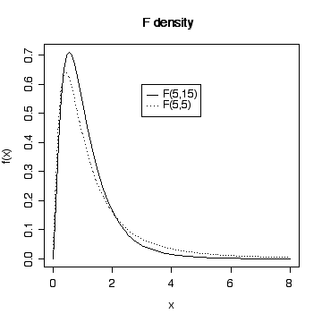
> xgr <- seq(0,8,length=90)
> plot(xgr, df(xgr,5,15), type = "l", lty = 1, xlab = "x", ylab ="f(x)")
> lines(xgr,df(xgr,5,5),lty=3)
> legend(3,.6,c("F(5,15)","F(5,5)"),lty=c(1,3))
> title("F density")
Question 2
(a) Analysis
Do EITHER simple linear regression OR
paired data analysis.
[Hand calculation 5; R calculation 5; Graph 3; Assumptions 3;
Conclusions 1]
Analysis as a Simple Linear Regression
> soil
sur sub diff
1 6.55 6.78 -0.23
2 5.98 6.14 -0.16
3 5.59 5.80 -0.21
4 6.17 5.91 0.26
5 5.92 6.10 -0.18
6 6.18 6.01 0.17
7 6.43 6.18 0.25
8 5.68 5.88 -0.20
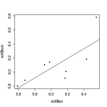
> plot(soil$sur,soil$sub,pch=19)
> fitsoil <- lm(sub~sur,data=soil)
> abline(fitsoil)
 > summary(fitsoil)
Call:
lm(formula = sub ~ sur, data = soil)
Residuals:
Min 1Q Median 3Q Max
-0.26473 -0.17263 0.03719 0.09778 0.34110
Coefficients:
Estimate Std. Error t value Pr(>|t|)
(Intercept) 1.8854 1.4416 1.308 0.2388
sur 0.6952 0.2375 2.927 0.0264 *
---
Signif. codes: 0 `***' 0.001 `**' 0.01 `*' 0.05 `.' 0.1 ` ' 1
Residual standard error: 0.2117 on 6 degrees of freedom
Multiple R-Squared: 0.5882, Adjusted R-squared: 0.5196
F-statistic: 8.57 on 1 and 6 DF, p-value: 0.02637
> anova(fitsoil)
Analysis of Variance Table
Response: sub
Df Sum Sq Mean Sq F value Pr(>F)
sur 1 0.38409 0.38409 8.57 0.02637 *
Residuals 6 0.26891 0.04482
---
Signif. codes: 0 `***' 0.001 `**' 0.01 `*' 0.05 `.' 0.1 ` ' 1
Assumptions
- Independence (Can't test);
- Normality (Could look at residuals, but not enough points;
however, data do appear to be more or less symmetrically
distributed above and below the fitted line.);
- Homoscedasticity (Variance seems to be about the same along
the line.)
- Linearity (Can't test, no repeated x-values.)
Conclusions
There is some evidence (P = 0.026) that the subsoil pH varies with surface pH. Surface pH could be used to predict subsoil pH but R-squared = 0.59 is not large so the prediction would be subject to error.
Analysis as Paired-Data Differences
> hist(soil$diff,bor="red",col="green")

> t0 <- (mean(soil$diff)-0)/sqrt(var(soil$diff)/length(soil$diff))
> t0
[1] -0.4793321

> 2*pt(t0,length(soil$diff)-1)
[1] 0.6463151
95% confidence interval for the mean difference
> mean(soil$diff)+c(-1,1)*qt(0.975,7)*sqrt(var(soil$diff)/8)
[1] -0.2224937  0.1474937
Assumptions
- Independence (Can't test, locations are not in any serial
order so autocorrelation would not be an issue.);
- Normality (The histogram of differences does not look normal,
there is a central gap, but the sample is too small to assess
normality.).
Conclusions
There is no evidence (P = 0.65) that the mean subsoil pH differs
from the mean surface pH at any given location.
Graph
A dot plot, box plot or histogram would also be good.
> stem(soil$diff)

  The decimal point is 1 digit(s) to the left of the |

  -2 | 310
  -1 | 86
  -0 |
   0 |
   1 | 7
   2 | 56
(b) Design [4 marks]
Possible sources of variation: type of soil; whether soil has been
cultivated recently; whether lime has been applied to the surface
recently; whether fertilizer has been applied recently; soil
moisture; sampling tool; contamination of subsoil by surface soil
when sampling; analytical techniqes; quality assurance at the
analysis laboratory; etc.
(c) Sample Size [4 marks]
Using the variance of the differences from (a), we will need 209
observations.
> var(soil$dif)
[1] 0.04896429
> var(soil$diff)*(qnorm(.975)/.03)^2
[1] 208.9937
Question 3
[Hand calculation 5; R calculation 5;
Graph 4; CI for residual variance 4; Assumptions 4; Conclusions
1]
Analysis as a One-Factor Design
> marg
poly brand
1 14.1 I
2 13.6 I
3 14.4 I
4 14.3 I
5 12.8 P
6 12.5 P
7 13.4 P
8 13.0 P
9 12.3 P
10 16.8 M
11 17.2 M
12 16.4 M
13 17.3 M
14 18.0 M
15 18.1 F
16 17.2 F
17 18.7 F
18 18.4 F
> boxplot(split(marg$poly,marg$brand)[c("I","P","M","F")],
xlab="brand",ylab="PAPFUA (%)")
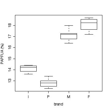 Note that a multiple dot plot would also be acceptable.
> anova(lm(poly~brand, data=marg))
Analysis of Variance Table
Response: poly
Df Sum Sq Mean Sq F value Pr(>F)
brand 3 84.764 28.255 103.77 8.428e-10 ***
Residuals 14 3.812 0.272
---
Signif. codes: 0 `***' 0.001 `**' 0.01 `*' 0.05 `.' 0.1 ` ' 1
95% Confidence Interval for the Residual Variance (either of the
following is acceptable)
> anova(lm(poly~brand, data=marg))$"Mean Sq"[2]

0.2722857

> anova(lm(poly~brand, data=marg))$"Mean Sq"[2]/c(qchisq(.975,14)/14,qchisq(.025,14)/14)
[1] 0.1459477 0.6772403
Assumptions
- Independence (Can't test);
- Normality (Could look at residuals, but not enough points;
however, data do appear to be more or less symmetrically
distributed within each brand.);
- Homoscedasticity (From the graph, variance seems to be about
the same for each brand.)
Conclusions
There is strong evidence (P << 0.01) that the percentage of
physiologically active polyunsaturated fatty acids varies between
brands.
Question 4
(a) Analysis
[Hand calculation 6; R calculation 6;
Graph 4; CI for residual variance 4; Assumptions 4; Conclusions
2]
> steel$ratef <- as.factor(steel$rate)
> steel
  rate loss ratef
1   14  280    14
2   18  350    18
3   18  330    18
4   40  470    40
5   43  500    43
6   43  490    43
7   43  470    43
8   45  560    45
9  112 1200   112
As a Simple Linear Regression
> fitsteel1 <- lm(loss~rate,data=steel)
> summary(fitsteel1)

Call:
lm(formula = loss ~ rate, data = steel)

Residuals:
   Min     1Q Median     3Q    Max
-57.92 -30.30  13.67  32.22  52.22

Coefficients:
            Estimate Std. Error t value Pr(>|t|)
(Intercept) 132.0732    25.2162   5.238  0.00120 **
rate          9.2057     0.5037  18.278 3.63e-07 ***
---
Signif. codes:  0 `***' 0.001 `**' 0.01 `*' 0.05 `.' 0.1 ` ' 1

Residual standard error: 41.69 on 7 degrees of freedom
Multiple R-Squared: 0.9795,	Adjusted R-squared: 0.9765
F-statistic: 334.1 on 1 and 7 DF,  p-value: 3.633e-07

> anova(fitsteel1)

Analysis of Variance Table

Response: loss
          Df Sum Sq Mean Sq F value    Pr(>F)
rate       1 580634  580634  334.08 3.633e-07 ***
Residuals  7  12166    1738
---
Signif. codes:  0 `***' 0.001 `**' 0.01 `*' 0.05 `.' 0.1 ` ' 1
As a One-Factor Design
> fitsteel2 <- lm(loss~ratef,data=steel)
> anova(fitsteel2)

Analysis of Variance Table

Response: loss
          Df Sum Sq Mean Sq F value    Pr(>F)
ratef      5 592133  118427  532.92 0.0001279 ***
Residuals  3    667     222
---
Signif. codes:  0 `***' 0.001 `**' 0.01 `*' 0.05 `.' 0.1 ` ' 1
As a Simple Linear Regression with Lack of Fit Test
> fitsteel <- lm(loss~rate+ratef,data=steel)
> anova(fitsteel)

Analysis of Variance Table

Response: loss
          Df Sum Sq Mean Sq  F value    Pr(>F)
rate       1 580634  580634 2612.852 1.649e-05 ***
ratef      4  11499    2875   12.937   0.03101 *
Residuals  3    667     222
---
Signif. codes:  0 `***' 0.001 `**' 0.01 `*' 0.05 `.' 0.1 ` ' 1

95% Confidence Interval for the Residual Variance (either of the following is acceptable)
Residual Variance - Not Assuming Linearity
The point estimate is 222.2, the 95% confidence interval is (71.3,
3089).
> anova(fitsteel)$"Mean Sq"[3]

222.2222

> anova(fitsteel)$"Mean Sq"[3]/c(qchisq(.975,3)/3, qchisq(.025,3)/3)
[1]   71.31342 3089.34773
Residual Variance - Assuming Linearity
The point estimate is 1738, the 95% confidence interval is (760,
7199).
> anova(fitsteel1)$"Mean Sq"[2]

1738.015

> anova(fitsteel1)$"Mean Sq"[2]/c(qchisq(.975,7)/7, qchisq(.025,7)/7)
[1]  759.7755 7199.4370

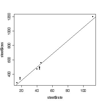
> plot(steel$rate,steel$loss,pch=19)
> abline(fitsteel1)
Assumptions
- Independence (Can't test);
- Normality (Could look at residuals, but not enough points;
however, data do appear to be more or less symmetrically
distributed about the line);
- Homoscedasticity (Distribution of points about the fitted line
seems to be about the same anywhere along the line.)
- Linearity (Some evidence of non-linearity by the lack of fit
test.)
Conclusions
There is evidence (P = 0.03) that the mean weight loss varies
non-linearly with SO2 deposition rate. We could stop
there. However, the line looks straight enough on the graph and
R2 = 0.98 is quite large, so the line should be usable for
linear interpolation. This justifies ignoring the lack of fit and we
can test the slope, which is highly significant (P << 0.01).

(b) Prediction [4 marks]
If we don't assume the linear relationship, we can't make a
prediction. However, the scatter of points about the fitted line is
quite tight, so a linear prediction should be valid. While rate = 43
is close to the observed data and so the prediction of 528
g/m2 should be reliable, rate = 80 is in a region where no
observations were taken so the prediction of 869 g/m2 is
less reliable.
> predict(fitsteel1,data.frame(rate=c(43,80)))
       1        2
527.9181 868.5288
Question 5
13-9 (p. 640).
(a) Analysis [Hand calculation 6; R
calculation 6]
Anneal temperature/time is coded as 1 = 900/60, 2 = 900/180, 3 =
950/60, 4 = 1000/15, 5 = 1000/30.
Polysilicon doping is coded 1 = 1*1020, 2 =
2*1020.
> fittrans <- lm(curr~doping*anneal, data=transistor)
> anova(fittrans)
Analysis of Variance Table

Response: curr
              Df  Sum Sq Mean Sq  F value    Pr(>F)
doping         1   1.442   1.442  25.2313 0.0005194 ***
anneal         4 124.238  31.059 543.5196 1.203e-11 ***
doping:anneal  4   0.809   0.202   3.5405 0.0477319 *
Residuals     10   0.571   0.057
---
Signif. codes:  0 `***' 0.001 `**' 0.01 `*' 0.05 `.' 0.1 ` ' 1
Conclusions [3 marks]
The interaction is (just) significant at the 5% level, so we
conclude that both polysilicon doping and anneal time/temperature
affect base current. Since the interaction is not highly
significant, we should also check the main effects; both polysilicon
doping and anneal time/temperature are highly significant.
(b) Interaction plots [4 marks]
> interactplot <-
function (y, facta, factb, xlab = deparse(substitute(factb)),
    ylab = deparse(substitute(y)), main = paste("Interaction plot by",
        deparse(substitute(facta))), ...)
{
    values <- sapply(split(y, facta:factb), mean)
    matplot(matrix(values, ncol = nlevels(facta)), type = "l",
        xlab = xlab, ylab = ylab, ...)
    title(main = main)
    legend(1, max(values), levels(facta), lty = 1:nlevels(facta),
        col = 1:nlevels(facta))
    invisible()
}

> attach(transistor)
> interactplot(curr,doping,anneal,ylab="current")
> interactplot(curr,anneal,doping,ylab="current")


(c) Analysis of residuals [6 marks]
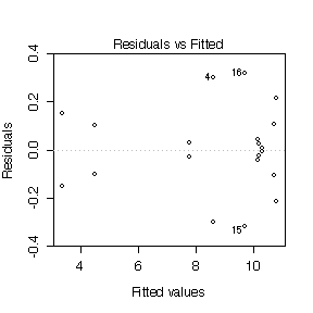
Since there are 20 residuals but only 10 degrees of freedom, there
are strong dependencies between the residuals and these show up as
symmetries in the plots. In particular, the plot of residuals versus
fitted values shows the positive residuals mirrored by negative
residuals and the negative quadrant of the normal QQ plot mirrors the
positive quadrant. Nonetheless, the scatter is reasonably random and
the normal QQ plot is reasonably straight, suggesting that the model
is adequate and the assumptions of the model are reasonably well
satisfied.
> plot(fittrans)


 > xgr <- seq(0,30,length=50)
> plot(xgr, dchisq(xgr, 2), type = "l", lty = 1, xlab = "x", ylab ="f(x)")
> lines(xgr,dchisq(xgr,5),lty=2)
> lines(xgr,dchisq(xgr,10),lty=3)
> legend(15,.4,c("2 df","5 df","10 df"),lty=1:3)
> title("Chi-square density")
 > xgr <- seq(0,8,length=90)
> plot(xgr, df(xgr,5,15), type = "l", lty = 1, xlab = "x", ylab ="f(x)")
> lines(xgr,df(xgr,5,5),lty=3)
> legend(3,.6,c("F(5,15)","F(5,5)"),lty=c(1,3))
> title("F density")

 > summary(fitsoil)
Call:
lm(formula = sub ~ sur, data = soil)
Residuals:
Min 1Q Median 3Q Max
-0.26473 -0.17263 0.03719 0.09778 0.34110
Coefficients:
Estimate Std. Error t value Pr(>|t|)
(Intercept) 1.8854 1.4416 1.308 0.2388
sur 0.6952 0.2375 2.927 0.0264 *
---
Signif. codes: 0 `***' 0.001 `**' 0.01 `*' 0.05 `.' 0.1 ` ' 1
Residual standard error: 0.2117 on 6 degrees of freedom
Multiple R-Squared: 0.5882, Adjusted R-squared: 0.5196
F-statistic: 8.57 on 1 and 6 DF, p-value: 0.02637
> anova(fitsoil)
Analysis of Variance Table
Response: sub
Df Sum Sq Mean Sq F value Pr(>F)
sur 1 0.38409 0.38409 8.57 0.02637 *
Residuals 6 0.26891 0.04482
---
Signif. codes: 0 `***' 0.001 `**' 0.01 `*' 0.05 `.' 0.1 ` ' 1
 Note that a multiple dot plot would also be acceptable.
> anova(lm(poly~brand, data=marg))
Analysis of Variance Table
Response: poly
Df Sum Sq Mean Sq F value Pr(>F)
brand 3 84.764 28.255 103.77 8.428e-10 ***
Residuals 14 3.812 0.272
---
Signif. codes: 0 `***' 0.001 `**' 0.01 `*' 0.05 `.' 0.1 ` ' 1