
If my instructions weren't clear enough, have a look at the spreadsheet I set up, then try to do it yourself. Having a graph automatically redrawn when you change the parameters is a neat feature of a spreadsheet. Click here to get my spreadsheet as an Excel 5.0/95 Workbook binary file. If you have trouble downloading the file, you can find it as ex02q1.xls in the folder Exercise_2 in the STAT 3N03 course folder in the BSB computer lab.
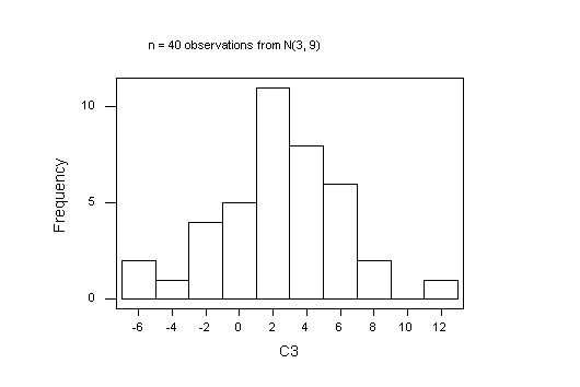
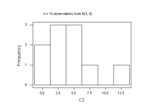
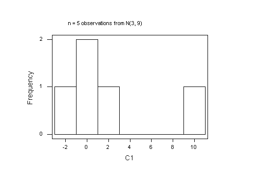
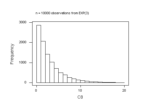
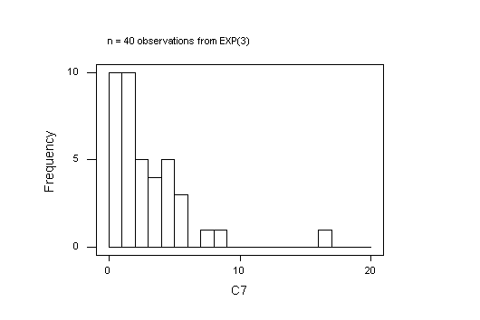
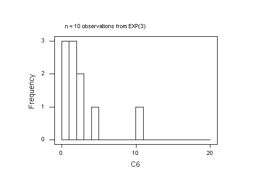
Here are the graphs I got; yours will be different, of course, because every sample of random random numbers will be unique. It is of interest to try a few samples at each sample size, just to see how different the histograms are. You can't say much about the shape of a distribution with fewer than 40 observations.
I have drawn these graphs in MINITAB. The default breaks (cut-points) will be diferent in R and that will also affect how the histograms look.

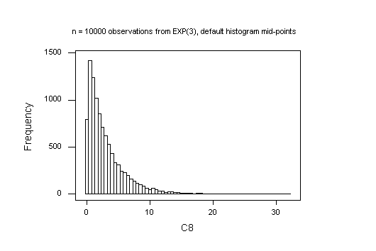
The default histogram in MINITAB is unsatisfactory here: MINITAB takes the first interval mid-point to be 0, so the first bar is too short because negative values are impossible for the Exponential distribution. To work around this, I forced the histogram to use cut-points defined at 0, 1, ..., 20.

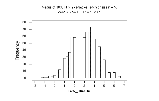
The MINITAB project ex02q3.mpj in the folder Exercise_2 in the STAT 3N03 course folder in the BSB computer lab shows my work for Normal and Exponential samples of size n = 5. The Normal samples are the 1000 rows of C1-C5 and the 1000 sample means are in C6. The theory predicts a mean of 3 and a standard deviation of 3/sqrt(5) = 1.34164 for the sampling distribution. The observed values, 2.9468 and 1.3177, respectively, are very close to that.
The Exponential samples are the 1000 rows of C11-C15 and the 1000 sample means are in C16. The theory predicts a mean of 3 and a standard deviation of 3/sqrt(5) = 1.34164 for the sampling distribution. The observed values, 2.9859 and 1.2909, respectively, are very close to that. However, the histogram shows that the sampling distribution is positively skewed and far from Normal. How close to Normal is it when n = 40?
