Statistics 3N03 - Assignment #3 Solutions
2001-12-03
Due: 2001-12-03 17:00
Use R to do the graphics on this assignment. Do the ANOVA calculations in R and with your calculator, and submit both. The text references are to Montgomery & Runger, Applied Statistics and Probability for Engineers, 2nd edition.
Full marks = 95
Question 1 [12 marks]
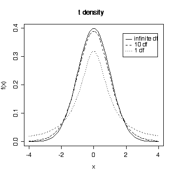
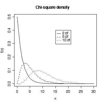
Use R to re-draw Figs. 8-11, 8-15 and 9-4 from the text.
> xgr <- seq(-4,4,length=50)
> plot(xgr, dnorm(xgr), type = "l", lty = 1, xlab = "x", ylab ="f(x)")
> lines(xgr,dt(xgr,10),lty=2)
> lines(xgr,dt(xgr,1),lty=3)
> legend(1.8,.38,c("infinite df","10 df","1 df"),lty=1:3)
> title("t density")
 > xgr <- seq(0,30,length=50)
> plot(xgr, dchisq(xgr, 2), type = "l", lty = 1, xlab = "x", ylab ="f(x)")
> lines(xgr,dchisq(xgr,5),lty=2)
> lines(xgr,dchisq(xgr,10),lty=3)
> legend(15,.4,c("2 df","5 df","10 df"),lty=1:3)
> title("Chi-square density")
 > xgr <- seq(0,8,length=90)
> plot(xgr, df(xgr,5,15), type = "l", lty = 1, xlab = "x", ylab ="f(x)")
> lines(xgr,df(xgr,5,5),lty=3)
> legend(3,.6,c("F(5,15)","F(5,5)"),lty=c(1,3))
> title("F density")

Question 2 [15 for hand calculation or computer calculation, +5 for both]
Analyze the following data from a study to determine the effect of air voids on percentage retained strength of asphalt. Air voids were controlled at three levels: low (2-4%), medium (4-6%) and high (6-8%). Give an appropriate graph. Give a 95% confidence interval for the residual variance. State any assumptions you make and do what you can to test the assumptions. State your conclusions.
Air Voids	Retained Strength (%)
Low        106    90   103    90    79    88
Medium      80    69    94    91    70    83
High        78    80    62    69    76    85
> asphalt <- data.frame(stren=c(106,90,103,90,79,88,80,69,94,91,70,83,78,80,62,69,76,85),
voids=rep(c("Low","Medium","High"),c(6,6,6)))
> asphalt
   stren  voids
1    106    Low
2     90    Low
3    103    Low
4     90    Low
5     79    Low
6     88    Low
7     80 Medium
8     69 Medium
9     94 Medium
10    91 Medium
11    70 Medium
12    83 Medium
13    78   High
14    80   High
15    62   High
16    69   High
17    76   High
18    85   High
> boxplot(split(asphalt$stren,asphalt$voids)[c("Low","Medium","High")],xlab="Air voids",ylab="Strength")

> anova(lm(stren~voids,data=asphalt))
Analysis of Variance Table

Response: stren
          Df  Sum Sq Mean Sq F value  Pr(>F)
voids      2  964.78  482.39    5.22 0.01902 *
Residuals 15 1386.17   92.41
---
Signif. codes:  0 `***' 0.001 `**' 0.01 `*' 0.05 `.' 0.1 ` ' 1
The 95% confidence interval for residual variance is:
> 92.41/c(qchisq(.975,15)/15,qchisq(.025,15)/15)
[1]  50.42674 221.35412
Assumptions:
- Independent observations - can't test.
- Normal distributions - can't test with such small samples but the box plots look reasonably symmetric.
- Homoscedasticity - we don't have a test to compare 3 variances, and the sample sizes are too small anyway, but the box plots look equal enough.
Conclusions:
There is evidence from these data (P = 0.02) that percentage retained strength depends on air voids over the range 2% to 8% air voids, with strength decreasing as the percent air voids increases.
Question 3 [20 for hand calculation or computer calculation, +5 for both]
A chemical reaction was run 9 times at different temperatures. The efficiency of the reaction was observed each time.
Temperature (°C)  10  30  20  50  40  10  20  10  40
Efficiency (%)    50  65  55  70  50  55  60  45  60
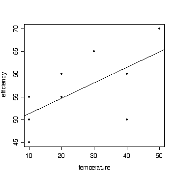
(a) Fit a straight line to the data by least squares, with efficiency as the dependent variable. Plot the data and the fitted line on a graph. Can efficiency be predicted as a linear function of temperature? Present your analysis in an ANOVA table with F-Tests for non-linearity and for the slope of the regression line. Give a 95% confidence interval for the residual variance. State your assumptions and your conclusions.
(b) Predict the efficiency to be obtained at 30°C, 60°C and 100°C. How reliable do you think your predictions are?
(a) Analysis
> react <- data.frame(temp=c(10,30,20,50,40,10,20,10,40),
eff=c(50,65,55,70,50,55,60,45,60))
> react
temp eff
1 10 50
2 30 65
3 20 55
4 50 70
5 40 50
6 10 55
7 20 60
8 10 45
9 40 60
> fitreact <- lm(eff~temp,data=react)
> coef(fitreact)
(Intercept) temp
48.0182927 0.3384146
> anova(fitreact)
Analysis of Variance Table
Response: eff
Df Sum Sq Mean Sq F value Pr(>F)
temp 1 208.689 208.689 5.0147 0.06014 .
Residuals 7 291.311 41.616
---
Signif. codes: 0 `***' 0.001 `**' 0.01 `*' 0.05 `.' 0.1 ` ' 1
> plot(react$temp,react$eff,xlab="temperature",ylab="efficiency")
> plot(react$temp,react$eff,xlab="temperature",ylab="efficiency",pch=19)
> abline(fitreact)
 > anova(lm(eff~temp+as.factor(temp),data=react))
Analysis of Variance Table
Response: eff
Df Sum Sq Mean Sq F value Pr(>F)
temp 1 208.689 208.689 7.4201 0.05277 .
as.factor(temp) 3 178.811 59.604 2.1192 0.24052
Residuals 4 112.500 28.125
---
Signif. codes: 0 `***' 0.001 `**' 0.01 `*' 0.05 `.' 0.1 ` ' 1
The confidence interval for the residual variance could be computed either from the regression anova (on 7 df), or from the regression anova with lack of fit (on 4 df):
> 41.616/c(qchisq(.975,7)/7,qchisq(.025,7)/7)
[1]  18.19249 172.38731

> 28.125/c(qchisq(.975,4)/4,qchisq(.025,4)/4)
[1]  10.09576 232.23718
Assumptions:
- Independence - can't test.
- Normality - can't test with such a small sample, could look at the distribution of the residuals in a larger sample.
- Homoscedasticity - can't test but the scatter of points about the line is reasonably constant along the line.
- Linearity - tested by the lack of fit test and accepted.
Conclusions:
There is no evidence from these data that the relationship is not linear over the range of temperatures studied (P = 0.24). Hence it is valid to test the slope, but the slope is not significantly different from zero (P = 0.053) so we do not have evidence that temperature affects efficiency over the range of temperatures studied.
(b) Predictions
> predict(fitreact,data.frame(temp=c(30,60,100)))
       1        2        3
58.17073 68.32317 81.85976

> mean(react$eff)
[1] 56.66667
If we accept the conclusion that temperature does not affect efficiency, the grand mean efficiency = 56.7% is the best prediction; the fitted line gives 58.2%, 68.2% and 81.9% efficiency at the three temperatures, respectively, but the predictions for 80' and 100' may not be valid because they are extrapolations and, in addition, we know that water boils at 100'.
Question 4 [15 for hand calculation or computer calculation, +5 for both]
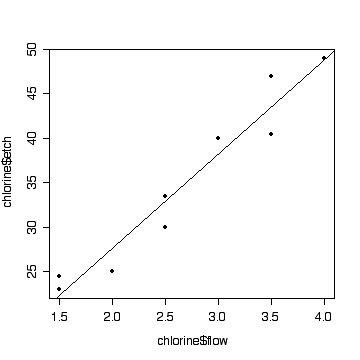
Analyze the following data from a study of ion-beam-assisted etching of aluminum with chlorine. The independent variable x is chlorine flow and the dependent variable y is the etch rate. Give an appropriate graph. State any assumptions you make and do what you can to test the assumptions. State your conclusions.
x    1.5    1.5    2.0    2.5    2.5    3.0    3.5    3.5    4.0
y   23.0   24.5   25.0   30.0   33.5   40.0   40.5   47.0   49.0
> chlorine <- data.frame(flow=c(1.5,1.5,2.0,2.5,2.5,3.0,3.5,3.5,4.0),
etch=c(23.0,24.5,25.0,30.0,33.5,40.0,40.5,47.0,49.0))
> chlorine
flow etch
1 1.5 23.0
2 1.5 24.5
3 2.0 25.0
4 2.5 30.0
5 2.5 33.5
6 3.0 40.0
7 3.5 40.5
8 3.5 47.0
9 4.0 49.0
> fitchlor <- lm(etch~flow,data=chlorine)
> coef(fitchlor)
(Intercept) flow
6.448718 10.602564
> anova(fitchlor)
Analysis of Variance Table
Response: etch
Df Sum Sq Mean Sq F value Pr(>F)
flow 1 730.69 730.69 112.76 1.438e-05 ***
Residuals 7 45.36 6.48
---
Signif. codes: 0 `***' 0.001 `**' 0.01 `*' 0.05 `.' 0.1 ` ' 1
> plot(chlorine$flow,chlorine$etch,pch=19)
> abline(fitchlor)
 > anova(lm(etch~flow+as.factor(flow),data=chlorine))
Analysis of Variance Table
Response: etch
Df Sum Sq Mean Sq F value Pr(>F)
flow 1 730.69 730.69 77.254 0.003103 **
as.factor(flow) 4 16.99 4.25 0.449 0.772619
Residuals 3 28.38 9.46
---
Signif. codes: 0 `***' 0.001 `**' 0.01 `*' 0.05 `.' 0.1 ` ' 1
Assumptions:
- Independence - can't test.
- Normality - can't test with such a small sample, could look at the distribution of the residuals in a larger sample.
- Homoscedasticity - can't test but the scatter of points about the line is reasonably constant along the line.
- Linearity - tested by the lack of fit test and accepted.
Conclusions:
There is no evidence from these data that the relationship is not linear over the range of chlorine flow studied (P = 0.77). Hence it is valid to test the slope, which is significantly different from zero (P = 0.003) so we have strong evidence that chlorine flow affects etch rate over the range of flows studied.
Question 5 [13 for hand calculation or computer calculation, +5 for both]
13-4 (p. 639).
> anode <- data.frame(dens=c(570,565,583,528,547,521,1063,1080,1043,988,1026,1004,565,510,590,526,538,532),
posit=factor(c(1,1,1,2,2,2,1,1,1,2,2,2,1,1,1,2,2,2)),
ftemp=factor(rep(c(800,825,850),c(6,6,6))))
> anode
   dens posit ftemp
1   570     1   800
2   565     1   800
3   583     1   800
4   528     2   800
5   547     2   800
6   521     2   800

7  1063     1   825
8  1080     1   825
9  1043     1   825
10  988     2   825
11 1026     2   825
12 1004     2   825
13  565     1   850
14  510     1   850
15  590     1   850
16  526     2   850
17  538     2   850
18  532     2   850
> fitanode <- lm(dens~posit*ftemp,data=anode)
> anova(fitanode)
Analysis of Variance Table

Response: dens
            Df Sum Sq Mean Sq  F value    Pr(>F)
posit        1   7160    7160   15.998  0.001762 **
ftemp        2 945342  472671 1056.117 3.253e-14 ***
posit:ftemp  2    818     409    0.914  0.427110
Residuals   12   5371     448
---
Signif. codes:  0 `***' 0.001 `**' 0.01 `*' 0.05 `.' 0.1 ` ' 1
> plot(fitanode)

(a) The hypotheses of interest are, first, that there is no interaction between firing temperature and position affecting the mean baked density, and, if that hypothesis is accepted, that there is no effect of firing temperature and that there is no effect of furnace position.
(b) The hypothesis of no interaction is accepted (P = 0.43) so we can test the main effects. The hypothesis that firing temperature does not affect the mean baked density is rejected (P << 0.001) as is the hypothesis that furnace position does not affect the mean baked density (P = 0.002).
(c) The plot of residuals versus fitted values shows an even scatter above and below the zero line, so the model appears to fit the data well.
 > xgr <- seq(0,30,length=50)
> plot(xgr, dchisq(xgr, 2), type = "l", lty = 1, xlab = "x", ylab ="f(x)")
> lines(xgr,dchisq(xgr,5),lty=2)
> lines(xgr,dchisq(xgr,10),lty=3)
> legend(15,.4,c("2 df","5 df","10 df"),lty=1:3)
> title("Chi-square density")
 > xgr <- seq(0,8,length=90)
> plot(xgr, df(xgr,5,15), type = "l", lty = 1, xlab = "x", ylab ="f(x)")
> lines(xgr,df(xgr,5,5),lty=3)
> legend(3,.6,c("F(5,15)","F(5,5)"),lty=c(1,3))
> title("F density")

 > anova(lm(stren~voids,data=asphalt))
Analysis of Variance Table
Response: stren
Df Sum Sq Mean Sq F value Pr(>F)
voids 2 964.78 482.39 5.22 0.01902 *
Residuals 15 1386.17 92.41
---
Signif. codes: 0 `***' 0.001 `**' 0.01 `*' 0.05 `.' 0.1 ` ' 1
  > anova(lm(eff~temp+as.factor(temp),data=react))
Analysis of Variance Table
Response: eff
Df Sum Sq Mean Sq F value Pr(>F)
temp 1 208.689 208.689 7.4201 0.05277 .
as.factor(temp) 3 178.811 59.604 2.1192 0.24052
Residuals 4 112.500 28.125
---
Signif. codes: 0 `***' 0.001 `**' 0.01 `*' 0.05 `.' 0.1 ` ' 1
  > anova(lm(etch~flow+as.factor(flow),data=chlorine))
Analysis of Variance Table
Response: etch
Df Sum Sq Mean Sq F value Pr(>F)
flow 1 730.69 730.69 77.254 0.003103 **
as.factor(flow) 4 16.99 4.25 0.449 0.772619
Residuals 3 28.38 9.46
---
Signif. codes: 0 `***' 0.001 `**' 0.01 `*' 0.05 `.' 0.1 ` ' 1