Statistics 3N03 - Assignment #3
2001-11-23
Due: 2001-12-03 17:00
Use R to do the graphics on this assignment. Do the ANOVA
calculations in R and with your calculator, and submit both. The text
references are to Montgomery & Runger, Applied Statistics and
Probability for Engineers, 2nd edition.
Question 1
Use R to re-draw Figs. 8-11, 8-15 and 9-4 from the
text. [Hint: See the example below.]
Question 2 [2000 Exam Q3]
Analyze the following data from a study to determine
the effect of air voids on percentage retained strength of asphalt.
Air voids were controlled at three levels: low (2-4%), medium (4-6%)
and high (6-8%). Give an appropriate graph. Give a 95% confidence
interval for the residual variance. State any assumptions you make
and do what you can to test the assumptions. State your conclusions.
Air Voids	Retained Strength (%)
Low        106    90   103    90    79    88
Medium      80    69    94    91    70    83
High        78    80    62    69    76    85
Question 3 [2000 Exam Q4]
A chemical reaction was run 9 times at different
temperatures. The efficiency of the reaction was observed each time.
Temperature (°C)  10  30  20  50  40  10  20  10  40
Efficiency (%)    50  65  55  70  50  55  60  45  60
(a) Fit a straight line to the data by least squares, with
efficiency as the dependent variable. Plot the data and the fitted
line on a graph. Can efficiency be predicted as a linear function of
temperature? Present your analysis in an ANOVA table with F-Tests for
non-linearity and for the slope of the regression line. Give a 95%
confidence interval for the residual variance. State your assumptions
and your conclusions.
(b) Predict the efficiency to be obtained at 30°C, 60°C
and 100°C. How reliable do you think your predictions are?
Question 4 [1999 Exam Q3]
Analyze the following data from a study of
ion-beam-assisted etching of aluminum with chlorine. The independent
variable x is chlorine flow and the dependent variable y is the etch
rate. Give an appropriate graph. State any assumptions you make and
do what you can to test the assumptions. State your conclusions.
x    1.5    1.5    2.0    2.5    2.5    3.0    3.5    3.5    4.0
y   23.0   24.5   25.0   30.0   33.5   40.0   40.5   47.0   49.0
Question 5
13-4 (p. 639). [Hint: see the example below.]
Hints:
The following examples will show you how to set up these problems
in R.
Re-draw Fig. 5-24 (p. 180)
> xgr <- seq(0,12,length=80)
> plot(xgr,dexp(xgr,2),type="l",lty=1,xlab="x",ylab="f(x)")
> lines(xgr,dexp(xgr,0.5),lty=2)
> lines(xgr,dexp(xgr,0.1),lty=3)
> legend(6,1.8,c("lambda = 2","lambda = 0.5","lambda = 0.1"),lty=1:3)
Note that I plotted the highest curve first, to set the limits on
the y-axis; I could also have done this by specifying ylim = c(0, 2)

Two-factor design: 13-3 (p. 639)
> tvtube <- data.frame(bright=c(280,290,285,230,235,240,300,310,295,260,240,235,290,285,290,220,225,230),
 glass=as.factor(rep(rep(1:2,rep(3,2)),3)), phosphor=as.factor(rep(1:3,rep(6,3))))
> tvtube
   bright glass phosphor
1     280     1        1
2     290     1        1
3     285     1        1
4     230     2        1
5     235     2        1
6     240     2        1
7     300     1        2
8     310     1        2
9     295     1        2
10    260     2        2
11    240     2        2
12    235     2        2
13    290     1        3
14    285     1        3
15    290     1        3
16    220     2        3
17    225     2        3
18    230     2        3
> anova(lm(bright~glass*phosphor, data=tvtube))
Analysis of Variance Table

Response: bright
               Df  Sum Sq Mean Sq  F value    Pr(>F)
glass           1 14450.0 14450.0 273.7895 1.259e-09 ***
phosphor        2   933.3   466.7   8.8421  0.004364 **
glass:phosphor  2   133.3    66.7   1.2632  0.317801
Residuals      12   633.3    52.8
---
Signif. codes:  0 `***' 0.001 `**' 0.01 `*' 0.05 `.' 0.1 ` ' 1
Simple Linear Regression with Lack of Fit: Example 10-9 (p. 467)
> exten9 <- data.frame(x=c(1,1,2,3.3,3.3,4,4,4,5,5.6,5.6,5.6,6,6,6.5,6.9),
 y=c(2.3,1.8,2.8,1.8,3.7,2.6,2.6,2.2,2,3.5,2.8,2.1,3.4,3.2,3.4,5))
> exten9
     x   y
1  1.0 2.3
2  1.0 1.8
3  2.0 2.8
4  3.3 1.8
5  3.3 3.7
6  4.0 2.6
7  4.0 2.6
8  4.0 2.2
9  5.0 2.0
10 5.6 3.5
11 5.6 2.8
12 5.6 2.1
13 6.0 3.4
14 6.0 3.2
15 6.5 3.4
16 6.9 5.0
> exten9$xf <- as.factor(exten9$x)
> exten9
     x   y  xf
1  1.0 2.3   1
2  1.0 1.8   1
3  2.0 2.8   2
4  3.3 1.8 3.3
5  3.3 3.7 3.3
6  4.0 2.6   4
7  4.0 2.6   4
8  4.0 2.2   4
9  5.0 2.0   5
10 5.6 3.5 5.6
11 5.6 2.8 5.6
12 5.6 2.1 5.6
13 6.0 3.4   6
14 6.0 3.2   6
15 6.5 3.4 6.5
16 6.9 5.0 6.9
Analysis as a simple linear regression:
> anova(lm(y~x,data=exten9))
Analysis of Variance Table

Response: y
          Df Sum Sq Mean Sq F value  Pr(>F)
x          1 3.4928  3.4928  6.6645 0.02174 *
Residuals 14 7.3372  0.5241
---
Signif. codes:  0 `***' 0.001 `**' 0.01 `*' 0.05 `.' 0.1 ` ' 1
Analysis as a one-factor design:
> anova(lm(y~xf,data=exten9))
Analysis of Variance Table

Response: y
          Df Sum Sq Mean Sq F value Pr(>F)
xf         8 7.7933  0.9742  2.2456 0.1515
Residuals  7 3.0367  0.4338
Analysis as a simple linear regression with a test for lack of
fit:
> anova(lm(y~x+xf,data=exten9))
Analysis of Variance Table

Response: y
          Df Sum Sq Mean Sq F value  Pr(>F)
x          1 3.4928  3.4928  8.0514 0.02513 *
xf         7 4.3005  0.6144  1.4162 0.32882
Residuals  7 3.0367  0.4338
---
Signif. codes:  0 `***' 0.001 `**' 0.01 `*' 0.05 `.' 0.1 ` ' 1
Since the lack of fit is not significant, we look further at the
simple linear regression model:
> fitexten9 <- lm(y~x,data=exten9)
> summary(fitexten9)

Call:
lm(formula = y ~ x, data = exten9)

Residuals:
     Min       1Q   Median       3Q      Max
-1.04505 -0.39160 -0.08988  0.34722  1.51873

Coefficients:
            Estimate Std. Error t value Pr(>|t|)
(Intercept)   1.6967     0.4730   3.587  0.00298 **
x             0.2586     0.1002   2.582  0.02174 *
---
Signif. codes:  0 `***' 0.001 `**' 0.01 `*' 0.05 `.' 0.1 ` ' 1

Residual standard error: 0.7239 on 14 degrees of freedom
Multiple R-Squared: 0.3225,	Adjusted R-squared: 0.2741
F-statistic: 6.665 on 1 and 14 DF,  p-value: 0.02174

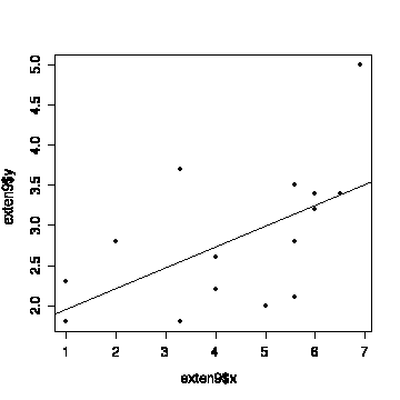
> plot(exten9$x,exten9$y,pch=19)
> abline(fitexten9)

Of course, we should have looked at the graph before starting any
analysis!

