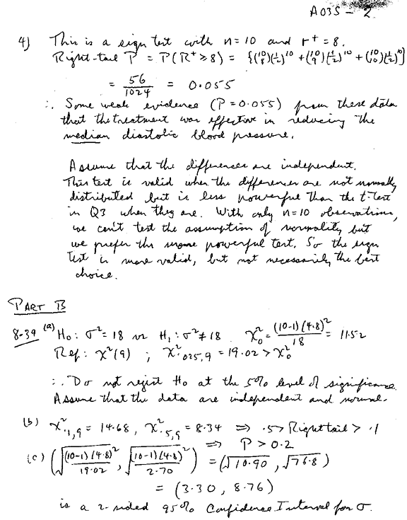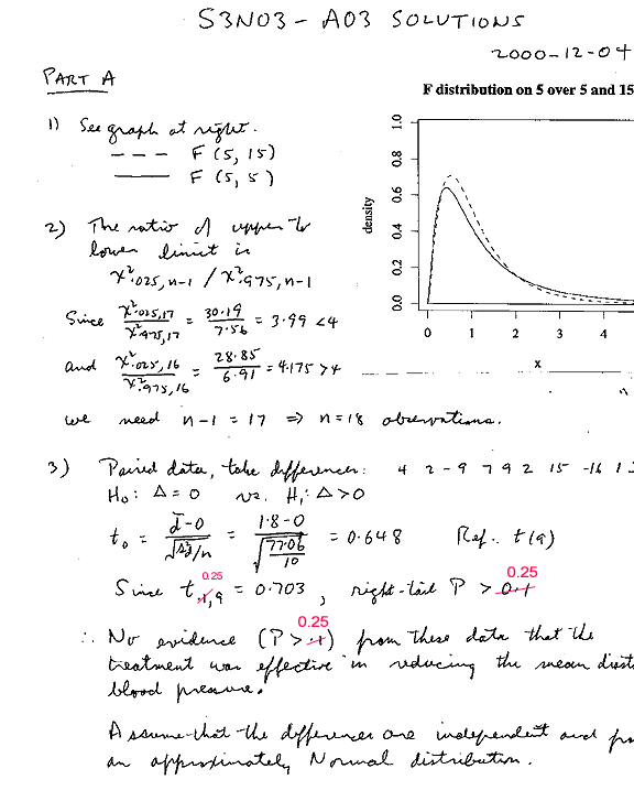
Part A, Q3
"Since t0.25,9 = 0.703, right-tail P > 0.25. No evidence ( P > 0.25) from these data..."
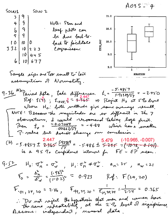
Part B, Q9-36(a)
"Ref.: t(6); t0.025,6 = 2.447" The conclusion remains the same.


I have done this exercise in R. The data have been read into a data frame object rocket.
> rocket
   strength   age
1   2158.70 15.50
2   1678.15 23.75
3   2316.00  8.00
4   2061.30 17.00
5   2207.50  5.00
6   1708.30 19.00
7   1784.70 24.00
8   2575.00  2.50
9   2357.90  7.50
10  2277.70 11.00
11  2165.20 13.00
12  2399.55  3.75
13  1779.80 25.00
14  2336.75  9.75
15  1765.30 22.00
16  2053.50 18.00
17  2414.40  6.00
18  2200.50 12.50
19  2654.20  2.00
20  1753.70 21.50
(a) Plot strength against age. The relationship looks reasonably linear.
> plot(rocket$age, rocket$strength)
(b) Use lm() to fit a simple linear regression and store the result in the object rocket.slr. Display the result to see the fitted slope and intercept.
> rocket.slr <- lm(strength~age, data=rocket)
> rocket.slr

Call:
lm(formula = strength ~ age, data = rocket)

Coefficients:
(Intercept)          age
    2625.39       -36.96
Add the fitted line to the plot.
> abline(rocket.slr)
(c) Use the fitted regression coefficients to estimate the mean strength when age = 20.
> coef(rocket.slr)
(Intercept)         age
  2625.3855    -36.9618
> coef(rocket.slr)[1]+coef(rocket.slr)[2]*20
(Intercept)
   1886.150
(d) Plot the fitted values against the observed strengths, for each observation in the data set, and compare this plot to a diagonal line through the origin. If the relationship were perfectly deterministic, the points would lie exactly along the diagonal. Here the points are more or less evenly scattered around the diagonal, indicating that age is a reasonable choice of regressor variable.
> plot(rocket$strength, predict(rocket.slr))
> abline(0, 1)
(a) Compute the analysis of variance table for the regression. The regression is significant at the 1% level.
> anova(rocket.slr)
Analysis of Variance Table

Response: strength
          Df  Sum Sq Mean Sq F value    Pr(>F)
age        1 1522819 1522819  155.21 2.753e-10 ***
Residuals 18  176602    9811
---
Signif. codes:  0  `***'  0.001  `**'  0.01  `*'  0.05  `.'  0.1  ` '  1
(b) The summary of the fit shows the standard errors of the regression coefficients. The estimate of error variance is found in the ANOVA table, MSE = 9811 on 18 degrees of freedom.
> summary(rocket.slr)

Call:
lm(formula = strength ~ age, data = rocket)

Residuals:
    Min      1Q  Median      3Q     Max
-233.08  -52.54   28.73   66.13  106.22

Coefficients:
            Estimate Std. Error t value Pr(>|t|)
(Intercept) 2625.385     45.347   57.90  < 2e-16 ***
age          -36.962      2.967  -12.46 2.75e-10 ***
---
Signif. codes:  0  `***'  0.001  `**'  0.01  `*'  0.05  `.'  0.1  ` '  1

Residual standard error: 99.05 on 18 degrees of freedom
Multiple R-Squared: 0.8961,     Adjusted R-squared: 0.8903
F-statistic: 155.2 on 1 and 18 degrees of freedom,      p-value: 2.753e-10
(c) A 2-sided t-test on 18 d.f. of the hypothesis that slope = -30 is done using the standard error of the slope estimate shown in the summary above. Since P = 0.031 we do not reject the hypothesis at the 1% level of significance.
> (-36.962 - (-30))/2.967
[1] -2.346478
> 2*pt(-2.346478, 18)
[1] 0.03059935
(d) A 2-sided t-test on 18 d.f. of the hypothesis that slope = 0 was given in the summary above. Since P = 2.75e-10, we reject the hypothesis at the 1% level of significance.
(e) A right-sided t-test on 18 d.f. of the hypothesis that intercept = 2500 is done using the standard error of the intercept estimate shown in the summary above. Since P = 0.0063 we reject the hypothesis at the 1% level of significance.
> (2625.385 - 2500)/45.347
[1] 2.765012
> 1-pt(2.765012, 18)
[1] 0.006378428
Full marks = 75
PART A
1 [4], 2 [2], 3 [5], 5 [5].
PART B
8-39 a [3], b [1], c [3];
9-18 d [3];
9-19 a [3], b [1], c [2], d [7];
9-36 a [4], b [2];
9-52 [5];
10-12 a [4], b [3], c [1], d [4];
10-27 a [4], b [3], c [2], d [2], e [2].