[Binomial-Poisson plot 5, Binomial-Normal plot 5]
The Bin(72, 1/36) distribution has
mean = 72 * (1/36) = 2
variance = 72 * (1/36) (35/36) = 1.9444
standard deviation = sqrt(1.9444) = 1.39443
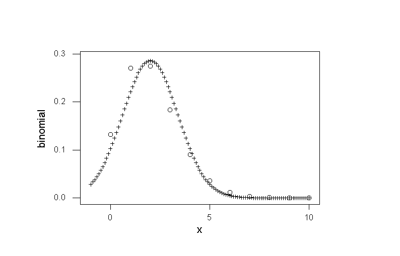
The first plot compares Bin(72, 1/36) (vertical lines) with Poisson(2) (open dots). The approximation is extremely close. A side-by-side bar plot (e.g. in Excel) would have been a better way to display this but I couldn't figure out how to do it in Minitab.

The second plot compares Bin(72, 1/36) (open dots) with N(2, 1.9444) (+), using overlay plots. The distributions are close but the approximation is very rough. We don't expect the approximation to be good here, since the mean is < 5.

Here are the same distributions, but I used vertical lines for the Binomial and a "line annotation" to add the Normal density as a smooth curve.

PART B - Question 2
[Simulation 8, approximating Normal 4, graph 3]
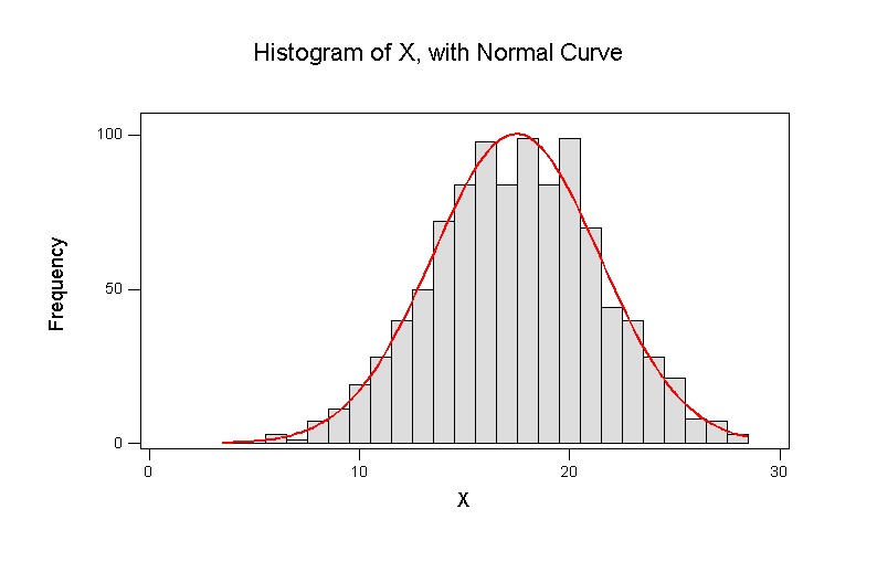
Here is the MINITAB session I ran to set up the discrete distribution (probability 1/6 at each of 1, 2, 3, 4, 5, 6, to simulate one die), then simulate 1000 rolls of 5 dice, compute the total score for each roll, and put the 1000 scores on a histogram with the approximating Normal.
From the formulas derived in 4-112, with a = 1 and b = 6, we have mean = 3.5 and variance = 35/12 = 2.916666 for the score on a single die. Hence for the total score on 5 independent dice
mean = 5 * 3.5 = 17.5
variance = 5 * 35/12 = 175/12 = 14.58333
standard deviation = sqrt(14.58333) = 3.8188
so the approximating Normal distribution is N(17.5, 14.58333).
The simulation gave a sample mean of 17.466 and a sample standard deviation of 3.9707, which are close to the theoretical values. Of course, your simulation results will be close but not exactly the same as mine or anyone else's.
You could compare the histogram of scores with the N(17.5, 14.58333).at the true mean and variance, or the fitted curve N(17.466, 3.97072); I used the default Minitab plot which shows the fitted Normal.
MTB > Set c8
DATA> 1( 1 : 6 / 1 )1
DATA> End.
MTB > Set c9
DATA> 6( 1 : 1 / 1 )1
DATA> End.
MTB > Let c9 = c9/6
MTB > Random 1000 c1-c5;
SUBC> Discrete 'y' 'prob'.
MTB > RSum c1-c5 c6.
MTB > Mean 'X'.
Mean of X
Mean of X = 17.466
MTB > StDev 'X'.
Standard Deviation of X
Standard deviation of X = 3.9707
MTB > Let k1 = 35/2
MTB > Let k2 = SQRT(5*35/12)
MTB > prin k1, k2
Data Display
K1 17.5000
K2 3.81881
MTB > Describe 'X';
SUBC> GNHist.
Descriptive Statistics: X

Variable N     Mean    Median  TrMean  StDev  SE Mean
X        1000  17.466  18.000  17.474  3.971  0.126
Variable  Minimum  Maximum  Q1      Q3
X         6.000    28.000   15.000  20.000

Histogram (with Normal Curve) of X
