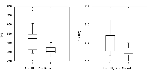
The stem-leaf plot wasn't specifically asked for, but it is the quickest way to sort the data for the box plots, and it is better than the box plots for assessing normality. Plotted side-by-side, the stem-leaf plots are as good as the box plots for comparing the two groups.
LHD                     Normal
Stem: hundreds          Stem: hundreds

2 85                    2 45,70,90
3 10,25,75              3 00,00,10,40,50,60
4 50,50,60,95           4 05
5
6 15
7 60

x_bar1 =   452.5        x_bar2 =  317.0
s12    = 21495.8333     s22    = 2217.777
s1     =   146.6146     s2     =   47.093

U Outliers     760      U Outliers
UH+1.5*HS      750      UH+1.5*HS     440
U Inlier       615      U Inlier      405
UH             495      UH            350
Median         450      Median        305
LH             325      LH            290
L Inlier       285      L Inlier      245
LH-1.5*HS       70      LH-1.5*HS      70
L Outliers              L Outliers
HS             170      HS             60
It is easy to re-draw the box plots on a log scale, but the log transformation doesn't help to equalize the variances in this example.

F-TEST FOR EQUALITY OF VARIANCES (TWO-SIDED TEST)
F0 = (21495.8333) / (2217.7777) = 9.6925; Reference Distribution is F(9,9).
The F tables have F(8,9) and F(12,9) but not F(9,9). The quick way to get the P-value here is to see that F8,9,0.995 = 6.69 and F12,9,0.995 = 6.23. Since F0 = 9.69 is bigger than both of these, we know that the area to the right of F0 under the F(9,9) density is less than 0.005, hence the two=sided P < 2 (0.005) = 0.01.
If we really wanted to, we could use interpolation to get
F9,9,0.995 = 6.69 + 0.25 (6.23 - 6.69) = 6.58
and interpolate between F8,9,0.999 = 10.37 and F12,9,0.999 = 9.57 to get
F9,9,0.999 = 10.37 + 0.25 (9.57 - 10.37) = 10.17;
then, since 6.58 < F0 < 10.17 we have that the two-sided P-value lies between 0.01 and 0.002.
Either way, there is evidence (P < 0.01) that the variances are not equal, so we should not assume that s12 = s22.
Unequal-variances t (page 272):
t0 = 2.7825, d' = 10.8; since t11,0.99 < t10,0.99 = 2.764, we find P < 2 (0.01) = 0.02.
Equal-variances t (page 259):
sp2 = 108.88, on 18 degrees of freedom, and t0 = 2.7825; t18,0.99 = 2.552.
Hence P < 2 (0.01) = 0.02
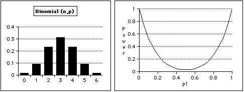
Since for Bin(6, 0.5) we have f(0) = f(6) = 0.0156, the two-sided test that is as close as possible to 5% is to reject when x = 0 or x = 6; the size of the test is then a = 2 (0.0156) = 0.0313.
Power = g(p1) = P(X = 0 | p1 ) + P(X = 6 | p1) = (1 - p1)6 + p16
The power curve shows that with n = 6, we do not have a good chance of detecting when p <> 0.5 unless p is about 0.1 or smaller, or about 0.9 or larger.

Q3
If it is true that the treatment is no different from the control, and this hypothesis is tested independently many times, then 5% of all the results will be Type I errors. That is, 5% of all the studies will lead to the false conclusion that the treatment is different from the control. But these will be only studies that get published, so anyone doing a literature search will find only evidence that the treatment is significantly different from the control.
If all the tests are two-sided, then on average half of the published results will show the treatment is better than the control and half will show that it is worse, so there is a chance that a thorough literature search will suggest that the treatment is not different from the control.
Q4
OR_hat = {(75)(73)}/{(53)(44)} = 2.34777 log(OR_hat) = 0.85347
Var_hat(log(OR_hat)) = 1/75 + 1/53 + 1/44 + 1/73 = 0.06863
z0.995 = 2.576
99% CI for log(OR) = 0.85347 ± (2.576)sqrt(0.06863)
= 0.85347 ± 0.67483
= (0.17864, 1.52830)
99% CI for OR = (exp(0.17864), exp(1.52830)) = (1.1956, 4.6103)
Hence we are 99% confident that the odds of remission are between 20% and 361% higher with the experimental treatment than with the control treatment.
Q1
Q2
Q3
Q4