 > mean(hosp$duration)
[1] 8.6
> mean(hosp$duration)+qnorm(.975)*(4/sqrt(25))
[1] 10.16797
> mean(hosp$duration)-qnorm(.975)*(4/sqrt(25))
[1] 7.032029
> mean(hosp$duration)
[1] 8.6
> mean(hosp$duration)+qnorm(.975)*(4/sqrt(25))
[1] 10.16797
> mean(hosp$duration)-qnorm(.975)*(4/sqrt(25))
[1] 7.032029> hosp<-read.table("Rosner\\Data\\hospital.dat")
> dimnames(hospital)[[2]]<-c("id","duration","age","sex","temp1","wbc1","antib","bact","serv")
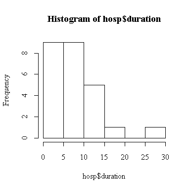
> hist(hosp$duration)
 > mean(hosp$duration)
[1] 8.6
> mean(hosp$duration)+qnorm(.975)*(4/sqrt(25))
[1] 10.16797
> mean(hosp$duration)-qnorm(.975)*(4/sqrt(25))
[1] 7.032029
> mean(hosp$duration)
[1] 8.6
> mean(hosp$duration)+qnorm(.975)*(4/sqrt(25))
[1] 10.16797
> mean(hosp$duration)-qnorm(.975)*(4/sqrt(25))
[1] 7.032029
The point estimate of mean duration of stay is 8.6 days. The 2-sided 95% confidence interval for mean duration is (7.03, 10.17) days, assuming that the standard deviation is 4 days.
> z0 <- (mean(hosp$duration) - 5)/(4/sqrt(25))
> z0
[1] 4.5
> 1 - pnorm(z0)
[1] 3.397673e-06
The p -value for a right-tailed z-test is very highly significant (P = 3e-6), so we reject the hypothesis and conclude that the mean duration of stay is greater than 5 days.
Next, compute the sample variance, the 2-sided 5% critical values and the test statistic to test the hypothesis that the standard deviation is 4 (i.e. that the variance is equal to 16). The Reference Distribution is chi-square on 25 - 1 = 24 degrees of freedom.
> var(hosp$duration)
[1] 32.66667
> c(qchisq(.025,24),qchisq(.975,24))
[1] 12.40115 39.36408
> 24*var(hosp$duration)/16
[1] 49
Since the test statistic lies in the rejection region, to the right of the upper limit, we reject the hypothesis at the 5% level of significance.
You weren't asked to find a p-value or a confidence interval, but they are given here for completeness.
Since the test statistic chisq0 = 49 is in the right tail of the chi-square distribution on 24 degrees of freedom, the two-sided p-value is twice the right-tail area. (How do we know it is in the right tail?)
> 2*(1-pchisq(49,24))
[1] 0.003788472
This is highly significant, so we reject the hypothesis. The 2-sided 95% confidence interval for the variance is given by
> c(24*var(hosp$duration)/qchisq(.975,24), 24*var(hosp$duration)/qchisq(.025,24))
[1] 19.91664 63.21994
that is, (19.92, 63.22), which does not include 16, so the hypothesis that the variance is 16 is rejected at the 5% level of significance.
If we don't assume a value for the standard deviation, we can use the sample standard deviation instead, and the Reference Distribution is the t-distribution (on 24 degrees of freedom) instead of the normal distribution.
> mean(hosp$duration)+qt(.975,24)*sqrt(var(hosp$duration)/25)
[1] 10.95923
> mean(hosp$duration)-qt(.975,24)*sqrt(var(hosp$duration)/25)
[1] 6.240767
The confidence interval (6.24, 10.96) is wider than the one above for two reasons: the t critical point is very slightly larger than the normal point, and the sample standard deviation is much larger than the standard deviation we had assumed.
> t0 <- (mean(hosp$duration) - 5)/sqrt(var(hosp$duration)/25)
> t0
[1] 3.149344
> 1 - pt(t0,24)
[1] 0.002170311
The p -value is much larger than before, but still highly significant, so our conclusion is unchanged.
Note that while we can use R much like a calculator, typing out the formulas, many common tests like the t-test are found in the ctest library.
> library(ctest)
> t.test(hosp$duration,alt="greater",mu=5)

         One Sample t-test

data:  hosp$duration
t = 3.1493, df = 24, p-value = 0.002170
alternative hypothesis: true mean is greater than 5
95 percent confidence interval:
 6.644299       NA
sample estimates:
mean of x
      8.6
Note all the information that t.test() returns, including the upper 95% confidence interval for mean duration.
Since we rejected the hypothesis that standard deviation is 4 days, all of the calculations made under this assumption are invalid. However, the histogram shows that the distribution of duration is not normal, so the test of the standard deviation is invalid. Since n = 25 is large enough, we are reasonably confident that the t-based confidence intervals and tests are valid.
Don't be confused by all the percents in the problem. Note that the 60% is never used, and the others are plus or minus percentage points ( D1 = 2%, s = 2.6%) and the significance level (5%) and Type II Error rate (1%) for the test. The calculation is
> ((qnorm(.975)+qnorm(.99))*2.6/2)^2
[1] 31.04947
> so at least 32 observations would be required. We have to assume that the distribution of concentration is close to normal; why would this assumption be questionable if the hypothesized concentration were 1% instead of 60% and the other figures remained the same?
If you sample randomly and independently, the number of positive responses you will get is distributed Binomial(n, p) and you want to test the null hypothesis that p = 0.6. (When working with counted data, it is best to work with proportions rather than percentages.) In these terms, D1 = .02 and the variance of the response from a single subject is s2 = pq = (0.6)(0.4) = .24. The calculation gives
> ((qnorm(.975)+qnorm(.99))*sqrt(.24)/0.02)^2
[1] 11023.48
where n = 11024 is certainly large enough for the normal approximation to the binomial to apply.
If this sample size is too large, you could lessen your requirements by increasing b or D1, or both, but you can't decrease the variance as it is determined by p.
> ((qnorm(.975)+qnorm(.9))*sqrt(.24)/0.02)^2
[1] 6304.454
> ((qnorm(.975)+qnorm(.9))*sqrt(.24)/0.03)^2
[1] 2801.979
Now we are no longer just planning the study, we have data.
> p <- 1623/3000
> p
[1] 0.541
> p + qnorm(.975)*sqrt(p*(1-p)/3000)
[1] 0.5588317
> p - qnorm(.975)*sqrt(p*(1-p)/3000)
[1] 0.5231683
so the 95% confidence interval for percent support is (52.3%, 55.9%).
By trial and error, we find that 22 df is the smallest df for which the ratio is less than 5, so the answer is n = 22+1 = 23. Note that the question specified 99% confidence.
> qchisq(.995,20)/qchisq(.005,20)
[1] 5.380372
> qchisq(.995,21)/qchisq(.005,21)
[1] 5.153454
> qchisq(.995,22)/qchisq(.005,22)
[1] 4.951644
Here are three different ways to compute the paired t-test in R. Note that the paired test is really a one-sample test, as it uses only the sample of differences. Why is the independent-samples t-test not valid for this example?
> ad <- valid$acff-valid$acdr
> length(ad)
[1] 173
> t0 <- mean(ad)/sqrt(var(ad)/length(ad))
> t0
[1] -0.02350511
> 2*(1-pt(abs(t0),length(ad)-1))
[1] 0.9812746
> t.test(valid$acff,valid$acdr,paired=T)

         Paired t-test

data:  valid$acff and valid$acdr
t = -0.0235, df = 172, p-value = 0.9813
alternative hypothesis: true difference in means is not equal to 0
95 percent confidence interval:
 -0.987287  0.964050
sample estimates:
mean of the differences
            -0.01161850

> t.test(valid$acff-valid$acdr)

         One Sample t-test

data:  valid$acff - valid$acdr
t = -0.0235, df = 172, p-value = 0.9813
alternative hypothesis: true mean is not equal to 0
95 percent confidence interval:
 -0.987287  0.964050
sample estimates:
  mean of x
-0.01161850
The assumptions are that the differences are independent, which we can't test because the observations are not in any particular order, and sufficiently close to normal. We can assess normality from a histogram:
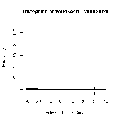
Overall, the histogram is reasonably symmetric, but, compared to a normal distribution, has a higher central peak and long, thin tails. Remembering previous analyses of these data, this is because both scores are much more variable when the level of consumption is high. This explains why the t-test is not significant.
Of more concern is the fact that the two middle bars of the histogram are far from equal, there are about twice as many small negative differences as there are small positive differences, suggesting that at low levels of consumption the food frequency questionnaire tends to report lower scores than the diet record. The t-test is dominated by a small number of very large differences and does not pick this up.
The sign test (Sect. 9.2, p. 333) is appropriate here. Count up the number of positive, negative and zero differences and apply Equation 9.2 on p. 335 to test the hypothesis that the difference is equally likely to be positive or negative, that is, that the median difference is 0. This formula uses the normal approximation to the binomial, with a continuity correction.
There are 55 positive differences and 102 negative differences for a total of 157 non-zero differences.
> sum(ad>0)
[1] 55
> sum(ad<0)
[1] 102
> sum(ad==0)
[1] 16
> 2*pnorm((55-(157/2)+.5)/sqrt(157/4))
[1] 0.0002414146
The result is very highly significant. The conclusion from the sign test is that the median difference is not zero, the food frequency questionnaire is more likely to report a lower level of alcohol consumption than the diet record. Because there are relatively few large differences, the sign test is dominated by the small differences. The only assumption required is independence of the differences.
If you are working on a computer, you don't need the normal approximation to the binomial, you can compute the p-value exactly. The test statistic is 55 and the Reference Distribution is Bin(157, 0.5). Since the test statistic is in the left tail, the p-value is twice the left tail probability.
> 2*pbinom(55,157,.5)
[1] 0.000218765
Note that the value computed by the normal approximation (with continuity correction) is very close to this exact value.
Begin by entering the data. The best format is a data frame with all the weights in one column, plus a column of treatment indicators. Compute some basic statistics and a comparative box plot.
> pods <- data.frame(wt=c(1.76,1.45,1.03,1.53,2.34,1.96,1.79,1.21,
+ .49,.85,1,1.54,1.01,.75,2.11,.92),treat=factor(c(rep("I",8),rep("U",8))))
> pods
     wt treat
1  1.76     I
2  1.45     I
3  1.03     I
4  1.53     I
5  2.34     I
6  1.96     I
7  1.79     I
8  1.21     I
9  0.49     U
10 0.85     U
11 1.00     U
12 1.54     U
13 1.01     U
14 0.75     U
15 2.11     U
16 0.92     U

> sapply(split(pods$wt,pods$treat),mean)
      I       U
1.63375 1.08375

> sqrt(sapply(split(pods$wt,pods$treat),var))
        I         U
0.4198958 0.5097881

> boxplot(split(pods$wt,pods$treat))
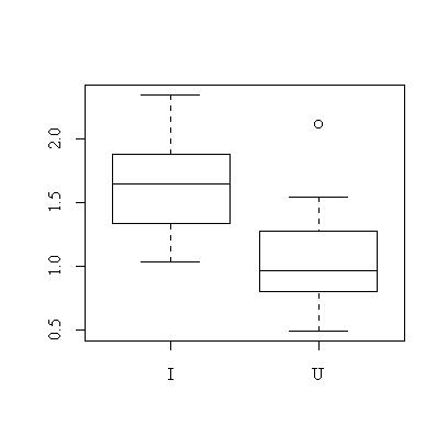
It is quite clear from the box plot that pods of the inoculated plants tend to be heavier.
> pwti<-pods$wt[pods$treat=="I"]
> pwtu<-pods$wt[pods$treat=="U"]

> mean(pwti)-qt(.975,7)*sqrt(var(pwti)/8)
[1] 1.282708
> mean(pwti)+qt(.975,7)*sqrt(var(pwti)/8)
[1] 1.984792
The 95% confidence interval for mean pod weight in the inoculated group is (1.28, 1.98) g.
> mean(pwtu)-qt(.975,7)*sqrt(var(pwtu)/8)
[1] 0.6575565
> mean(pwtu)+qt(.975,7)*sqrt(var(pwtu)/8)
[1] 1.509944
The 95% confidence interval for mean pod weight in the untreated group is (0.65, 1.51) g.
Even though the separate confidence intervals for the two treatments overlap, the confidence interval for the difference in means (0.05, 1.05) g, computed below, does not include zero. This is because calculations on the difference in means take into account the fact that both means are not likely to be at extremes of their distributions at the same time.
> t.test(pwti,pwtu,var.equal=T)

          Two Sample t-test

data:  pwti and pwtu
t = 2.3554, df = 14, p-value = 0.03361
alternative hypothesis: true difference in means is not equal to 0
95 percent confidence interval:
 0.04918173 1.05081827
sample estimates:
mean of x mean of y
  1.63375   1.08375
The two-sided p-value = 0.034 for the independent-samples t-test, so we can reject the hypothesis that the means are equal at the 5% level of significance.
Here are the calculations as you would do them "by hand"; note the calculation of the pooled standard deviation, sp.
> sp <- sqrt((7*var(pwti)+7*var(pwtu))/14)
> sp
[1] 0.4670099
> t0 <- (mean(pwti)-mean(pwtu))/(sp*sqrt((1/8)+(1/8)))
> t0
[1] 2.355411
> 2*(1-pt(abs(t0),14))
[1] 0.03361488
If you didn't have a computer to compute the p-value, you would use Table 5 on p. 757, with 14 degrees of freedom. Since t0 = 2.355 lies between t0.975,14 = 2.145 and t0.99,14 = 2.624, the area to the right of t0 is between 0.025 and 0.01 so you know that the 2-sided p-value lies between 0.05 and 0.02.
We have assumed that the distribution of pod weight is close to normal in each treatment group. The sample sizes are too small to test this but the box plot does not indicate any problems. We have also assumed that the variances are the same in both treatment groups. This can be tested:
> var.test(pwti,pwtu)

         F test to compare two variances

data:  pwti and pwtu
F = 0.6784, num df = 7, denom df = 7, p-value = 0.6214
alternative hypothesis: true ratio of variances is not equal to 1
95 percent confidence interval:
 0.1358239 3.3886856
sample estimates:
ratio of variances
         0.6784279
Here are the calculations as you would do them "by hand":
> F0 <- var(pwti)/var(pwtu)
> F0
[1] 0.6784279
> 2*pf(F0,7,7)
[1] 0.6214363
Note that the F0 statistic is in the left tail, so the 2-sided p-value is computed as twice the left tail area. Since p-value = 0.62, which is not significant, we say that there is no evidence from these data that the variances are not equal.
If we had to do this F-test without the help of a computer, using the tables in the book, take the reciprocal of F0, 1/F0 = 1.474, to put the statistic into the right tail. From Table 9 on p. 762, F0.90,7,7 = 2.78 > 1.474, so the area to the right of 1.474 is > 0.1, so we conclude that the 2-sided p-value > 0.2, which is not significant.
Check that pods$treat is a factor. (In this case, the levels are indicated by characters, not numbers, so it was automatically made a factor when the data frame was created, but we can check anyway.) Then use the linear model function lm() to fit wt modeled as a linear function of treat and use anova() to display the result in the standard anova table format. Note that by specifying data=pods we can refer to variables in the data frame by their names in the data frame, without the prefix pods$. Note also that lm() expects the data in the way we entered it: a data frame with all the pod weights in one column and all the treatment indicators in another.
> is.factor(pods$treat)
[1] TRUE
> anova(lm(wt~treat, data=pods))
Analysis of Variance Table

Response: wt
          Df Sum Sq Mean Sq F value  Pr(>F)
treat      1 1.2100  1.2100   5.548 0.03361 *
Residuals 14 3.0534  0.2181
---
Signif. codes:  0  `***'  0.001  `**'  0.01  `*'  0.05  `.'  0.1  ` '  1
The t-statistic was 2.3554 and 2.35542 = 5.5479 which is the F-statistic in the anova table. The p-values are the same for both tests. The result is declared "significant", indicated by one star.
The mean squared residual is 0.2181 on 14 degrees of freedom; sqrt(0.2181) = 0.46701 which agrees with the pooled standard deviation computed for the t-test.
Since the MSE = 0.2181 on 14 df, the required 95% confidence interval is given by
> c(14*0.2181/qchisq(0.975,14), 14*0.2181/qchisq(0.025,14))
[1] 0.1169036 0.5424673
Since the sample size was small, I typed it directly into a data frame, declaring the status variable to be a factor. Note that rep(1,7) gives 1, 1, 1, 1, 1, 1, 1, etc.
> mother <- data.frame(birthwt=c(7.5,6.2,6.9,7.4,9.2,8.3,7.6,
+ 5.8,7.3,8.2,7.1,7.8,5.9,6.2,5.8,4.7,8.3,7.2,6.2,6.2,6.8,5.7,
+ 4.9,6.2,7.1,5.8,5.4),smoker=factor(c(rep(1,7),rep(2,5),rep(3,7),rep(4,8))))

> mother
   birthwt smoker
1      7.5      1
2      6.2      1
3      6.9      1
4      7.4      1
5      9.2      1
6      8.3      1
7      7.6      1
8      5.8      2
9      7.3      2
10     8.2      2
11     7.1      2
12     7.8      2
13     5.9      3
14     6.2      3
15     5.8      3
16     4.7      3
17     8.3      3
18     7.2      3
19     6.2      3
20     6.2      4
21     6.8      4
22     5.7      4
23     4.9      4
24     6.2      4
25     7.1      4
26     5.8      4
27     5.4      4

> boxplot(split(mother$birthwt,mother$smoker),ylab="Birth Weight",xlab="Mother's Smoking Status")
The box plot tells the story so clearly that further analysis is hardly necessary: birth weights are very similar for babies of non-smoker (1) and ex-smoker (2) mothers, and much lower for babies of smokers (3, 4). Babies of heavy smokers (4: one or more packs per day) have only slightly lower birth weights than babies of light smokers (3: less than a pack a day). However, the analysis is not convincing without p-values.
> anova(lm(birthwt~smoker,data=mother))
Analysis of Variance Table

Response: birthwt
          Df  Sum Sq Mean Sq F value  Pr(>F)
smoker     3 11.6727  3.8909  4.4076 0.01371 *
Residuals 23 20.3036  0.8828
---
Signif. codes:  0  `***'  0.001  `**'  0.01  `*'  0.05  `.'  0.1  ` '  1
This result establishes that the means of the four groups are significantly different. (The text also shows how to establish which of the means are the most different but there isn't time to include those methods in the course.)
The estimate of residual variance is 0.8828 on 23 degrees of freedom, so the 95% confidence interval is (0.533, 1.737).
> c(23*0.8828/qchisq(0.975,23), 23*0.8828/qchisq(0.025,23))
[1] 0.533265 1.737119
This is a balanced two-factor design with replication. It can be fitted with lm(). The formula cover ~ paint*roller means fit all main effects and interactions for paint and roller; it is shorthand notation for cover ~ paint + roller + paint:roller, where the colon indicates interaction. Make sure that both paint and roller are factors in the data frame.
> latex
   paint roller cover
1      1      1   454
2      1      1   460
3      1      2   446
4      1      2   440
5      2      1   446
6      2      1   445
7      2      2   444
8      2      2   449
9      3      1   439
10     3      1   432
11     3      2   442
12     3      2   443

> anova(lm(cover~paint*roller,data=latex))
Analysis of Variance Table

Response: cover
             Df  Sum Sq Mean Sq F value  Pr(>F)
paint         2 248.000 124.000 10.0541 0.01214 *
roller        1  12.000  12.000  0.9730 0.36203
paint:roller  2 234.000 117.000  9.4865 0.01387 *
Residuals     6  74.000  12.333
---
Signif. codes:  0  `***'  0.001  `**'  0.01  `*'  0.05  `.'  0.1  ` '  1
The interaction is significant (p-value = 0.014) so we conclude that mean coverage depends on which paint and roller combination is used. Because the interaction is significant, we do not test the main effects.
This analysis assumes that the observations are independent and normally distributed, and the variance s2 is the same within each paint-roller combination.
The estimate of the residual variance s2 is 12.333 on 6 degrees of freedom, so a 95% confidence interval is (5.12, 59.81).
> c(6*12.3333333/qchisq(0.975,6), 6*12.3333333/qchisq(0.025,6))
[1]  5.121329 59.805507
If we save the lm object from the fit, we can use it to plot graphs, calculate the ANOVA table, display the regression coefficients, etc.
> fitage <- lm(duration~age, data=hosp)
> summary(fitage)

Call:
lm(formula = duration ~ age, data = hosp)

Residuals:
   Min     1Q Median     3Q    Max
-7.469 -2.438 -1.058  1.187 19.461

Coefficients:
            Estimate Std. Error t value Pr(>|t|)
(Intercept)  4.33762    2.52406   1.719   0.0991 .
age          0.10336    0.05523   1.871   0.0741 .
---
Signif. codes:  0  `***'  0.001  `**'  0.01  `*'  0.05  `.'  0.1  ` '  1

Residual standard error: 5.439 on 23 degrees of freedom
Multiple R-Squared: 0.1321,     Adjusted R-squared: 0.09441
F-statistic: 3.502 on 1 and 23 degrees of freedom,      p-value: 0.07406

> anova(fitage)
Analysis of Variance Table

Response: duration
          Df Sum Sq Mean Sq F value  Pr(>F)
age        1 103.60  103.60  3.5022 0.07406 .
Residuals 23 680.40   29.58
---
Signif. codes:  0  `***'  0.001  `**'  0.01  `*'  0.05  `.'  0.1  ` '  1

> plot(hosp$age,hosp$duration)
> abline(fitage)
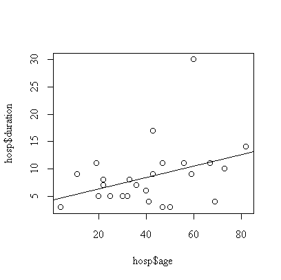
The effect of age is not significant (p-value = 0.074, calculated either from the t-test on the coefficient or F-test on the regression).
If you were using the F-tables in Rosner, you would see that F1,20,0.90 = 2.97, F1,20,0.95 = 4.35, F1,30,0.90 = 2.88, F1,30,0.95 = 4.17; the observed F0 = 3.5022 on 1 over 23 d.f. lies between the 0.90 and 0.95 points in either case, the test is right-tailed, so 0.05 < p-value < 0.10. Or, using the t-tables, t23,0.95 = 1.714 and t23,0.975 = 2.069; the observed t0 = 1.871 lies between the 0.95 and 0.975 points, the test is 2-tailed, so 0.05 < p-value < 0.10. The tests are identical, of course, since there is 1 d.f. in the numerator and of the F-test and hence F0 = t02.
We assume that the effect of age is linear , that the observations are independent, and that the distribution of duration of stay at a given age is normal with constant variance. The graph indicates one outlier, subject #7 with a 30-day stay. The analysis could be repeated with this subject removed or with the transformation to log(duration) to reduce the effect of the outlier.
It is tempting to conclude that the regression is "almost significant" but as you will see in Assignment #3, reducing the effect of the outlier reduces the slope and increases the p-value.
> fittemp1 <- lm(duration~temp1, data=hosp)
> summary(fittemp1)

Call:
lm(formula = duration ~ temp1, data = hosp)

Residuals:
   Min     1Q Median     3Q    Max
-5.089 -3.919 -1.421  1.916 19.422

Coefficients:
            Estimate Std. Error t value Pr(>|t|)
(Intercept) -154.505    168.585  -0.916    0.369
temp1          1.659      1.715   0.968    0.343

Residual standard error: 5.723 on 23 degrees of freedom
Multiple R-Squared: 0.03911,    Adjusted R-squared: -0.00267
F-statistic: 0.9361 on 1 and 23 degrees of freedom,     p-value: 0.3433

> anova(fittemp1)
Analysis of Variance Table

Response: duration
          Df Sum Sq Mean Sq F value Pr(>F)
temp1      1  30.66   30.66  0.9361 0.3433
Residuals 23 753.34   32.75
> plot(hosp$temp1, hosp$duration)
> abline(fittemp1)
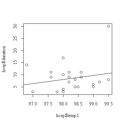
Although the fitted line has positive slope = 1.659, it is not significantly different from zero (p-value = 0.34).
We assume that the effect of first temperature is linear , that the observations are independent, and that the distribution of duration of stay at a given first temperature is normal with constant variance. The graph indicates one outlier, subject #7 with a 30-day stay. The analysis could be repeated with this subject removed or with the transformation to log(duration) to reduce the effect of the outlier.
> dimnames(hosp)[[2]]
[1] "id" "duration" "age" "sex" "temp1" "wbc1"
[7] "antib" "bact" "serv"
> cor(hosp[,c(2,3,5,6)])
duration age temp1 wbc1
duration 1.0000000 0.3635209 0.1977573 -0.0467783
age 0.3635209 1.0000000 -0.3816794 -0.3693244
temp1 0.1977573 -0.3816794 1.0000000 0.4235478
wbc1 -0.0467783 -0.3693244 0.4235478 1.0000000
> pairs(hosp[,c(2,3,5,6)])
 > fitatw <- lm(duration~age+temp1+wbc1, data=hosp)
> summary(fitatw)
Call:
lm(formula = duration ~ age + temp1 + wbc1, data = hosp)
Residuals:
Min 1Q Median 3Q Max
-7.6535 -3.6776 -0.7611 1.4346 14.6667
Coefficients:
Estimate Std. Error t value Pr(>|t|)
(Intercept) -330.21378 176.46026 -1.871 0.0753 .
age 0.14396 0.05939 2.424 0.0245 *
temp1 3.39045 1.79770 1.886 0.0732 .
wbc1 -0.05508 0.37942 -0.145 0.8860
---
Signif. codes: 0 `***' 0.001 `**' 0.01 `*' 0.05 `.' 0.1 ` ' 1
Residual standard error: 5.237 on 21 degrees of freedom
Multiple R-Squared: 0.2654, Adjusted R-squared: 0.1605
F-statistic: 2.529 on 3 and 21 degrees of freedom, p-value: 0.08486
> anova(fitatw)
Analysis of Variance Table
Response: duration
Df Sum Sq Mean Sq F value Pr(>F)
age 1 103.60 103.60 3.7779 0.06546 .
temp1 1 103.92 103.92 3.7892 0.06508 .
wbc1 1 0.58 0.58 0.0211 0.88596
Residuals 21 575.90 27.42
---
Signif. codes: 0 `***' 0.001 `**' 0.01 `*' 0.05 `.' 0.1 ` ' 1
> plot(hosp$duration,fitted(fitatw))
> abline(0,1)
> plot(fitatw)
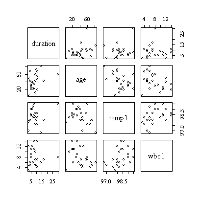
The correlation matrix and pairs plot show that the relations between the variables are very weak, so we would not expect a strong model.
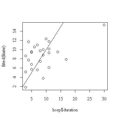
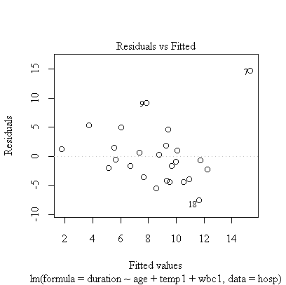
Note the call plot(fitatw); the default plot() of a fit object like fitatw gives a series of plots including the ones requested here. If you wanted to work with the residuals, you could use either residuals(fitatw) or fitatw$residuals to get them.
Age and first temperature are almost significant as predictors of duration of stay, but first WBC is not significant. The residual plot shows that the 7th observation is an outlier and the analysis should be repeated with the outlier removed, or with duration of stay log-transformed.
> anova(lm(duration~temp1+age+wbc1, data=hosp))
Analysis of Variance Table

Response: duration
          Df Sum Sq Mean Sq F value  Pr(>F)
temp1      1  30.66   30.66  1.1180 0.30236
age        1 176.86  176.86  6.4490 0.01907 *
wbc1       1   0.58    0.58  0.0211 0.88596
Residuals 21 575.90   27.42
---
Signif. codes:  0  `***'  0.001  `**'  0.01  `*'  0.05  `.'  0.1  ` '  1
Age is significant (p-value = 0.02) as a linear predictor of duration of stay, but only after adjusting for first temperature, i.e. if age is fitted after first temperature. Why will the plots in Q1 also apply to this model?
Because there are repeated x-values in the data, we can define flow as a factor (flowf at 6 distinct levels) as well as as a quantitative variable (flow).
> etch <- data.frame(flow=c(1.5,1.5,2,2.5,2.5,3,3.5,3.5,4),
+ rate=c(23,24.5,25,30,33.5,40,40.5,47,49))
> etch$flowf <- as.factor(etch$flow)

> etch
  flow rate flowf
1  1.5 23.0   1.5
2  1.5 24.5   1.5
3  2.0 25.0     2
4  2.5 30.0   2.5
5  2.5 33.5   2.5
6  3.0 40.0     3
7  3.5 40.5   3.5
8  3.5 47.0   3.5
9  4.0 49.0     4
> fitflow <- lm(rate~flow, data=etch)
> summary(fitflow)

Call:
lm(formula = rate ~ flow, data = etch)

Residuals:
    Min      1Q  Median      3Q     Max
-3.0577 -2.6538  0.5449  1.7436  3.4423

Coefficients:
            Estimate Std. Error t value Pr(>|t|)
(Intercept)   6.4487     2.7946   2.308   0.0544 .
flow         10.6026     0.9985  10.619 1.44e-05 ***
---
Signif. codes:  0  `***'  0.001  `**'  0.01  `*'  0.05  `.'  0.1  ` '  1

Residual standard error: 2.546 on 7 degrees of freedom
Multiple R-Squared: 0.9415,     Adjusted R-squared: 0.9332
F-statistic: 112.8 on 1 and 7 degrees of freedom,       p-value: 1.438e-005
The regression ANOVA shows that flow is very highly significant as a predictor of etch rate, assuming a linear relationship with independent normal error and homoscedasticity.
> anova(fitflow)
Analysis of Variance Table

Response: rate
          Df Sum Sq Mean Sq F value    Pr(>F)
flow       1 730.69  730.69  112.76 1.438e-05 ***
Residuals  7  45.36    6.48
---
Signif. codes:  0  `***'  0.001  `**'  0.01  `*'  0.05  `.'  0.1  ` '  1
The one-factor ANOVA shows that flow is very highly significant as a predictor of etch rate, assuming independent normal error and homoscedasticity but not assuming a linear relationship.
> anova(lm(rate~flowf, data=etch))
Analysis of Variance Table

Response: rate
          Df Sum Sq Mean Sq F value  Pr(>F)
flowf      5 747.68  149.54   15.81 0.02296 *
Residuals  3  28.37    9.46
---
Signif. codes:  0  `***'  0.001  `**'  0.01  `*'  0.05  `.'  0.1  ` '  1
> plot(etch$flow,etch$rate)
> abline(fitflow)

We can also fit flow, then flowf, to get the following ANOVA table.
> anova(lm(rate~flow+flowf, data=etch))
Analysis of Variance Table

Response: rate
          Df Sum Sq Mean Sq F value   Pr(>F)
flow       1 730.69  730.69  77.254 0.003103 **
flowf      4  16.99    4.25   0.449 0.772619
Residuals  3  28.38    9.46
---
Signif. codes:  0  `***'  0.001  `**'  0.01  `*'  0.05  `.'  0.1  ` '  1
You will recognize the regression sum of squares (730.69) from the simple linear regression ANOVA and the residual or "pure error" sum of squares (28.38) from the one-factor ANOVA; the lack-of-fit sum of squares (flowf in the table) is calculated as the difference between the regression residual sum of squares and the one-factor residual sum of squares.
The conclusion is that flow affects etch rate linearly (flowf p-value = 0.77, so there is no evidence of non-linearity) and highly significantly (flow p-value = 0.003).
The assumptions are independence (can't test), normality (too few observations to test but the scatter about the fitted line is reasonably symmetric), homoscedasticity (to few observations to test but the scatter about the fitted line is reasonably consistent) and linearity (tested by the lack -of-fit F test, the hypothesis of linearity was not rejected).
If you want to investigate the residuals about the fitted line (to assess normality, for example) you can get them with either residuals(fitflow) or fitflow$residuals.
Since we have accepted the simple linear regression model, we can use the fitted line to predict the etch rate when flow = 1.75. With your pocket calculator, you could do this once you have the slope and intercept or, if you still have the data in the calculator, simply by entering 1.75 and pushing the "y-hat" button (y with a ^ over it). In R, the results of the simple linear regression fit are in fitflow, so you can use
> predict(fitflow,data.frame(flow=1.75))
[1] 25.00321
which is a bit clumsy because the new value of flow has to be supplied in a data frame.
Be careful if you are trying to extrapolate out of the range of the data; the model predicts an etch rate of 6.45 when flow = 0, for example, but the fitted line might not apply there.
You have two estimates of the residual variance; the simple linear regression ANOVA gives a mean squared residual of 6.480311 on 7 df, while the one-factor ANOVA gives 9.458333 on 3 df. The corresponding 95% confidence intervals for the true residual variance are
> c(6.480311/(qchisq(0.975,7)/7), 6.480311/(qchisq(0.025,7)/7))
[1]  2.832876 26.843603
> c(9.458333/(qchisq(0.975,3)/3), 9.458333/(qchisq(0.025,3)/3))
[1]   3.035277 131.490358
The first interval (2.83, 26.84) is preferable; it is much tighter because it is based on more degrees of freedom. The only additional assumption is that the straight line model applies and that was validated by the test for nonlinearity.
In case you are wondering how I got the mean squares to more decimal places than the ANOVA shows, I used
> anova(fitflow)$"Mean Sq"[[2]]
[1] 6.480311
to extract the second "Mean Sq" in the "Mean Sq" column of the ANOVA table.
> library(ctest)
> pulmonary <- matrix(c(78,371,26,295,1111,106),ncol=2)
> dimnames(pulmonary) <- list(c("Hispanic","Black","Other"), c("Study","NCICAS"))

> chisq.test(pulmonary)

	 Pearson's Chi-squared test

data:  pulmonary
X-squared = 4.1603, df = 2, p-value = 0.1249

> chisq.test(pulmonary)$observed

         Study NCICAS
Hispanic    78    295
Black      371   1111
Other       26    106

> chisq.test(pulmonary)$expected

             Study    NCICAS
Hispanic  89.16709  283.8329
Black    354.27781 1127.7222
Other     31.55511  100.4449
Since all of the expected counts are much greater than 5, the chi-square test is valid. The result is not significant (p-value = 0.12) so there is no evidence from these data that the proportions of the three ethnic groups vary between the two studies.